As is usually the case with scientific buzz words in everyday parlance, in books, in the cinema, on TV, and on the internet – like energy – the meaning of the word dimension rarely aligns with what mathematicians and physicists understand it to be. This day and age it’s rather uncommon to not have been exposed to phrases such as ‘higher’ or ‘other dimensions’. It’s likely you’ve used them yourself once or twice in your life. In this episode, we’ll explore what mathematicians and physicists mean when they talk about dimensions, and, more interestingly, the spaces they yield.
Dimensions are not Universes
In science-fiction or even everyday lingo, the word ‘dimension’ is often synonymous with entire worlds, or realms or (pocket) Universes. For instance, aliens may have come from another dimension. Or souls or ‘essences’ dwelling on a ‘higher plane of existence’ in another ‘dimension of reality’ are spoken about.
On a regular basis, portals to other dimensions are opened from which exotic forms of matter and energy are extracted to benefit either the hero or the bad guy of the story.
It’s also a favourite way to travel great distances within our reality. Just hop through a dimensional portal and out you come, back into our reality, only thousand kilometres away from where you started. Occasionally, you may also travel in time by flying through other dimensions.
And, of course, other dimensions can be summoned into our own reality or, if the story goes that they have always been present inside our reality, they can be made visible by powerful minds. This is, again, alluding to dimensions being whole separate realms within our realm.
Figure 1. Doctor Stephen Strange (Benedict Cumberbatch) is about to step into the Mirror Dimension as summoned within (or next to) our reality by his mentor, the Ancient One (Tilda Swinton), in the 2016 film Doctor Strange of the wildly popular Marvel Cinematic Universe (MCU). License note. (Click to enlarge.)
This whole section was just to let you know that what is meant by dimensions in most science-fiction stories is not what is meant in mathematics and physics. They are not realms, realities, worlds or pocket Universes. If we were to refer to realms, realities, worlds, and Universes, we would just say realms, realities, worlds, and Universes, but not dimensions.
Ordinary spaces and dimensions
So, what do mathematicians and physicists mean when they talk about dimensions?
In many cases, they pertain to the actual directions you and I are able to travel in ordinary space. I prefer to think of birds and fish as gorgeous examples of being able to travel in all directions of space all by their own.
They can fly from your left to your right and vice versa (first direction). They can fly head-on towards you and whizz by over your head and fly further behind you and vice versa (second direction). And, obviously, they can fly up from underneath you and they can keep on flying to way above your face. And vice versa (third direction).
In many cases, all three directions are oriented perpendicularly with respect to each other. To use another word, they are orthogonal. All motion can be described as some combination of moving in these three orthogonal directions, i.e. orthogonal dimensions.
In high school we have gotten all too familiar with these three dimensions. We were tortured with finding distances between vertices of a cube along the edges, the sides, and straight through the block. Of course, this is what modern gadgets and cinematography refer to when they use the term 3D, three-dimensional. In some way or form, all three orthogonal dimensions are either taken advantage of or simulated in a virtual way.
Mathematically, the capability of travelling (or ‘transporting’) along these three orthogonal directions automatically give rise to a space, a topology, of some shape or form. Ordinary space is the space you and I are born in and have grown very much accustomed to.
So, while dimensions may give rise to spaces, they are definitely not the same. Besides, while one dimension by itself technically yields a topology, a space, it’s still a one-dimensional space, meaning, no three-dimensional bodies are able to traverse this without being torn apart.
Figure 2. In ordinary space, we have three dimensions in the $x$-direction, the $y$-direction, and the $z$-direction. In high school, we were to calculate the distance between points $O$ and $F,$ for instance.
Euclid and Descartes
A very informal definition of dimensions is the number of coordinates needed to locate an object (in a space of some kind). So, on a flat surface (a plane), such as a ceiling, you need two coordinates to locate a fly. A fly can be 2 metres away from the left wall (the first direction) and 3 metres away from the back wall (the second direction, perpendicular to the first direction). Its coordinates are therefore (2,3). Hence, a plane is two-dimensional.
In ordinary, three-dimensional space, we need three coordinates to locate a fly in a room. A fly can be 2 metres away from the left wall, 3 metres away from the back wall, and 1.5 metres up from the floor. Its coordinates are therefore (2,3,1.5).
This was one of René Descartes’s great insights while lying in bed late in the afternoon or so the story goes. Hence, these numbers are called Cartesian coordinates. Descartes was pivotal to the development of what we now call the Cartesian coordinate system.
The space to which these type of coordinates belong is called Euclidean space as the great Greek mathematician Euclid was the father of Euclidean or classical geometry.
I think I can safely say that Euclid and Descartes enabled mathematics teachers to torment us with a whole slew of homework in order for us to fully explore the realm of Euclidean space in both two- and three-dimensional Cartesian coordinate systems.
Figure 3. Home of Descartes in Utrecht, the Netherlands, where he wrote parts of his famous Discours de la Méthode. The house has been demolished. Nowadays, the place looks very different. (Click on the image for a link to the original Instagram post where you can also swipe for the photo of what is looks like today. Opens a new tab.)
Space and time
In real life, besides a position in ordinary space, you also need to specify when. Getting the coordinates to be inside an office located on the corner of two streets on the 24th floor (that’s the three dimensions of ordinary space right there) just isn’t enough. You also need a time-coordinate. When are you supposed to be there?
Einstein called the fact that you’re inside an office at a certain time an event. In other words, where, in ordinary, Cartesian coordinates, we talked about some thing being somewhere, Einstein had the insight to now only start talking about events taking place in terms of space and time, space-time – using space-time coordinates.
When Einstein introduced the special theory of relativity, the German mathematician Hermann Minkowski realised this theory could also be understood geometrically in a four-dimensional space-time, where time is taken to be the fourth dimension. We now call this space Minkowski space. Note that we’re using the word ‘space’ in a broader sense: it doesn’t just encompass ordinary spatial dimensions but it now also includes a dimension of time (and, for technical reasons, isn’t Euclidean).
By the way, another word mathematicians and physicists like to use is manifold. A manifold is a topological object which can take many shapes – such as a two-dimensional plane, a three-dimensional Euclidean space, four-dimensional Minkowski space or any other space you can mathematically think of.
In Einstein’s general theory of relativity (gravity), we still work with four-dimensional space-time, except the shape of the space isn’t Minkowskian any more. The shape of the space is warped, curved, and stretched. In the best theory of gravity we have to date, we work on a so-called pseudo-Riemannian manifold, named after the great German mathematician Bernhard Riemann. The dimensions are still all the directions you can take on this manifold, i.e. the minimum amount of coordinates you need to locate an event. However, in this case, they are not necessarily oriented perpendicularly with respect to one another.
Figure 4. In the film Interstellar (2014), director Christopher Nolan featured an object which had something to do with space and time. (Click to enlarge.) If you haven’t seen the film and still intend to, do not read this footnote:(beginfootnote)Astronaut Joseph Cooper (Matthew McConaughey) finds himself in this spatial representation of space-time. All four dimensions of particular events in the past, present, and future of a room in his house, chopped up into manageable time chunks, are mapped onto an object (called a Tesseract) inside of a black hole (where the roles of space and time are reversed) through which Cooper can transport himself freely. This enables him to trickle information into the events of his choosing. In the still image above, you see many instances of the same room of his house with his daughter at different positions in time (which is the equivalent of different positions in space for Cooper).(endfootnote). License note.
Four ordinary space dimensions
Imagine a Pac-Man living on the surface of a sphere. To them, the world is flat. If they were to travel straight on – and on and on and on – eventually, they would be quite surprised to find themselves returning to the point where they started.
Figure 5. Imagine being as flat as a Pac-Man, travelling on what seems to be a flat surface. You might be surprised to find you’d eventually end up where you started. If you had no knowledge of the three-dimensional concept of a sphere, that is. We do. We know that you’d return because that’s what a sphere – or a circle, for that matter – does to your path. But what about our Universe? What if we would travel billions and billions of years in a straight line through the Universe? Would we end up where we started? Could our Universe be some kind of hypersphere(beginfootnote)Yes, technically, it’s a glome, or an n-sphere, where $n=3,$ and the space it’s embedded in is $n=1$, not a hypersphere. Apologies to the mathematicians and physicists.(endfootnote)?
We, the three-dimensional beings most of us are, see them as a little surface, a shape, because we can see them ‘from above’, from the third dimension. We can also see how they’re travelling around the surface of a sphere. They don’t know what a sphere is. They only think of flat surfaces. To us, however, it’s quite logical they would eventually return to their point of origin.
Okay, so, back to our 3D world. Imagine we travelled in a spaceship, always in a straight line through the Universe. Now imagine, after billions of years, we end up where we started: Earth. What happened? Could our Universe be some kind of sphere, only four-dimensional?
While no experiment has proven the existence of a fourth spatial dimension (let alone five or six etc.), it is a wonderfully entertaining world for the mind to ponder about.
Just to be absolutely sure: time is not the fourth dimension we’re talking about here. We were talking space – spatial dimensions. Quite often these two get confused: four-dimensional space-time is three spatial dimensions plus one time-dimension while four-dimensional space is four spatial dimensions without time.
Abstract spaces
There’s another way in which dimensions and spaces are used by mathematicians and physicists. Imagine an object having several properties at once: a position (in ordinary space), motion, direction of that motion, temperature, colour. To describe the state of this object, you need more than just four space-time coordinates. Suppose, its space-time coordinates are (0,1,1,1), in other words, it exists at time $t=0$ at position $(x=1; y=1; z=1)$.
Did we describe the state of the whole object? No, we’re still missing some key properties here. It is in motion, so, it has a speed, say 10 m/s. That speed has a direction – this is why we say it has a velocity, which is speed and direction. Let’s say its velocity $v = -10 \text{ m/s},$ in other words, it has a speed of $10 \text{ m/s}$ to the left.
Let’s say its temperature is 273.15 Kelvin, which is 0 ℃ and 32 ℉. And its colour is pure white. So, how many numbers do we need to describe the object’s state fully? Exactly, seven numbers (we count ‘white’ as a number).
The coordinates (0,1,1,1,-10,273.15,white) are said to live in phase space, an abstract space where the properties of the object form the dimensions of that space. This particular phase space is seven-dimensional. Of course, that’s impossible to imagine, but mathematically, you can work very well with it.
We gave an unusual example to emphasise that dimensions needn’t be related to spatial and temporal positions. However, usually, phase spaces are indeed used in the context of position and momentum.
Figure 6. A sample trajectory through phase space is plotted near a so-called Lorenz attractor, a solution to the Lorenz system, which Edward Lorenz developed to model atmospheric convection. The colour of the solution fades from black to blue as time progresses, and the black dot shows a particle moving along the solution in time. The three-dimensional trajectory in phase space is shown from different angles to demonstrate its structure.
Another example of an abstract space is a so-called vector space where each coordinate does not just occupy a point in that space but that point also has a direction. An example of such a space is the velocity of wind. Each point in that space does not just have a value pertaining to the speed of the air and its location in ordinary space, it has a direction too.
In the previous post, Complex numbers: an introduction, an entirely new kind of number line was introduced. All the spaces we just mentioned could very well contain complex dimensions. In fact, most of the time, they do. Especially in quantum mechanics. Complex numbers make up abstract complex vector spaces where wave functions thrive. Hilbert space is where it’s at, most of the time.
The Standard model of quantum physics is based on groups of symmetrical transformations in complex space, called SU(3) $\times$ SU(2) $\times$ U(1). The S stands for special and denotes all possible transformations in complex space except for one particular kind. U(1) refers to a one-dimensional unitary circle group in the complex plane. The numbers indicate the number of dimensions in which these transformations take place. The number of dimensions of the entire system is much higher, though! The dimensionality of the abstract complex space which follows from a symmetry group such as SU(3) is $3^2-1=8.$ As you can see, compared to street corner vernacular, dimensions are very different in scientific context.
In general, we can say that every manifold is a space. This needn’t pertain to spatial space. The minimum amount of dimensions needed to construct a path to a point on that manifold is the dimensionality of that space.
There are so many more types of mathematical spaces, they’re too many to mention. Suffice to say, while they have nothing to do with our ordinary space – our real-world one, which we dwell in – all these abstract spaces are brilliant mathematical tools enabling us to do predictive calculations pertaining to phenomena taking place in our ordinary, real-world space.
String theories
An interesting beast among all of this is string theory. If you accept the premise that an elementary particle such as an electron is actually a spatially one-dimensional string vibrating in specific ways corresponding to the collection of properties of an electron, then more dimensions are automatically needed in order to describe all the particles in this way. Strings need a sufficient amount of freedom, degrees of freedom, to vibrate in unique ways to be able to encompass the entire zoo of elementary particles and their properties.
Figure 7. The basic building blocks of the entire Universe, according to string theory. Unfortunately, while the theory is mathematically consistent, it cannot yet be (and hasn’t been) proven to be correct in this Universe.
In various versions of the string theories, a varying number of dimensions are needed. These dimensions are spatial and invisible. Since we don’t experience these dimensions, it is hypothesised that they are extremely small and curled up. They’re not stretched out like our ordinary three spatial dimensions.
Or they are so large that to us they don’t affect us in any way noticeable. Just as the curvature of Earth did not affect us when we were little as the Earth is so big compared to our movements.
Unfortunately, the theory cannot be tested yet. For now it’s purely a mathematical exercise. Although many discoveries have been made in pure mathematics, no experiment has proven string theory to be true (string theory in all its variety, and I’m including superstring theories and M-theory here even though the hierarchy is the other way around). No extra dimensions have been found yet.
There’s one honourable mention that I’d like to make. It’s the Calabi-Yau manifold, or the Calabi-Yau space. In superstring theory the manifold is hypothesised to encompass six invisible extra dimensions for the theory to work. The manifold is three-complex-dimensional or six-real-dimensional. I like it because it looks cool.
None of this is proven; we seem to be stuck in this three-dimensional space with one direction of time. And, if you ask me, it’s likely that our three-dimensional space turns out to be a side product of something quantum.
Figure 8. A Calabi-Yau manifold, named after Eugenio Calabi and Shing-Tung Yau. This is a complex space with complex dimensions. It yields applications in theoretical physics, most notably in superstring theory, where the manifold has six dimensions. Though not experimentally proven to be existing in our world, they do yield fascinating mathematical possibilities and puzzles.
Spaces and dimensions
There are so many different spaces with a variety of dimensions that you’d need a whole slew of posts to describe them all properly.
What can we take away from all of this? Dimensions are not realms. In ordinary space, they are the directions in which objects can freely be transported. That’s three for our world.
If you model time as a dimension, then we live in a four-dimensional space-time world. Except that you can’t freely move in time as there’s only one direction(beginfootnote)Time is definitely going to be a whole separate set of posts. Can’t wait.(endfootnote).
Though many had hoped to find extra spatial dimensions, the largest experiment humankind has undertaken, the Large Hadron Collider at CERN, has not found a shred of evidence for them. Instead, it delivered convincing evidence that the current Standard Model of particle physicswithout extra dimensions is still correct.
Nevertheless, to describe and predict phenomena in our Universe, it is almost always helpful to model their properties as extra dimensions. This has nothing to do with there actually being extra dimensions – this is probably where popular and esoteric culture get their inspiration from – but has everything to do with being able to do calculations in the abstract world of mathematics.
In a previous post, for example, we assumed imaginary time as an extra dimension to mathematically derive a set of equations in the special theory of relativity. It doesn’t mean imaginary time is an actual extra dimension you can dip appendages or your consciousness into.
In string theories, actual extra spatial dimensions are required for the theories to work. None of them can be tested as of yet (and none of them have been tested nor proven). It remains to be a beautiful, mathematical construct, but only mathematical.
In future posts, we will be exploring geometry, pseudo-Riemannian manifolds, symmetry groups, and Hilbert space for loads more bits of maths and physics.
Licenses
The featured image in the title and Figures 1 are still images of Marvel Studio’s Doctor Strange (2014) and Figure 4 of Interstellar (2014), all copyrighted films. It is believed that screenshots may be exhibited under the fair use provision of United States copyright law.
Figure 6. Lorenz attractor animation by Dan Quinn under CC BY-SA 3.0
Probably the most famous equation on this planet is $E = mc^2$. Energy equals mass times the speed of light squared(beginfootnote)Usually, in mathematics, we leave out the multiplication sign ($\times$).(endfootnote). Usually, the formula is associated with Albert Einstein. This relationship between, energy, mass, and the speed of light, this equation, has a name: the mass-energy equivalence. Perhaps you’ve read or heard people explain that ‘Einstein taught us’, that mass is a form of energy, mass is frozen energy, mass can be converted into energy, and that, in the end, all matter is essentially pure energy.
The equation is, however, definitely not about all of that. At least, not in this Universe. Here, we will discuss the actual meaning of it. We think it’s time for disposing of some of the unnecessary obscurantism accompanying many popular explanations. We think the involved mathematicians and physicists of yore deserve better.
Albert Einstein (right) with Dutch physicist Paul Ehrenfest (left) and Ehrenfest’s son in Ehrenfest’s home in Leiden, The Netherlands.
Standing on the shoulders of giants
Einstein wasn’t the first to write down this very relationship between mass and energy. There were many others before him who, one way or the other, explored the connection between mass, energy, and velocity. However, most hypothesised that a mechanical mass increase was exclusively due to interactions with electromagnetic fields. They called it electromagnetic self-energy of some kind, giving rise to a form of electromagnetic mass (Miller, 1981; Okun, 1989). Einstein then showed that there was no need for such a concept and was the first to derive the relation correctly.
However, over the course of a few years, he published several derivations of the equation, none of which were literally written down as $E = mc^2$. You might not recognise them if you saw them. Furthermore, the versions he did write down, weren’t universally true.
Lastly, the famous equation isn’t the complete version. Usually, people only know the snazzy edition fitting on baseball caps. The full equation is valid in a more universal way and sometimes referred to by contemporary physicists as the ‘correct version’(beginfootnote)cf. https://youtu.be/mkiCPMjpysc(endfootnote). However, this one wasn’t first formulated by Einstein but by Paul Dirac (Eisberg & Resnick, 1974; Miller, 1981). We will get back to that.
Among others, these incredible minds have all derived and used some version of the famous equation before Einstein.
Energy is a mathematical idea
We should remind ourselves that energy isn’t any ‘thing’. As we mentioned in a previous article, it isn’t some invisible, immaterial, fluid-like ‘essence’ which everything is made of, within and behind the façade of the tangible world. Fork, no.
It has always been just a number, an accounting tool, an important and practical, mathematical concept, first proposed by the 17th century, German scholar Gottfried Wilhelm von Leibniz. How is it a mathematical concept? It’s the number you get when you multiply an object’s mass with its velocity squared(beginfootnote)Which was later calibrated to 1/2 times the mass times velocity squared.(endfootnote). It’s a pragmatic way of keeping the books on these two things.
Suppose, we have a billiard table with three billiard balls. We ignore any sort of friction. Imagine this isolated system of balls changing internally: the balls constantly collide and bounce off of the edge of the table. He assumed that what doesn’t change, is their mass. What does change, are their velocities. Leibniz then noticed that if you multiply for each ball its mass with its velocity squared, and summed all three products, that sum remained constant, irrespective of how the balls were bouncing in which direction, and how fast, at each point in time (until you changed something to the system by introducing a whack by a cue stick, for example).
This was the early formulation of what we now fanciful call the law of conservation of energy(beginfootnote)He called this product quantity vis viva, so, not even energy yet. Perhaps he was being poetic. Furthermore, Leibniz also had some fierce competition: his rival Newton had come up with a different quantity, a different way of keeping the books. He stated that the sum of the products of mass and velocity — just velocity, not velocity squared — remained constant. This is the law of conservation of momentum. Later, it was understood that the two laws were complimentary, not contradictory.(endfootnote), which, by the way, is true in a small enough patch of the Universe, such as Earth or the solar system, but in the context of the entire observable Universe, for instance, energy is not conserved. So, indeed, the law of conservation of energy is fundamental enough for us, Earthlings, and our physics experiments, however, contrary to what people usually think, in the grander scheme of the Universe, it’s not(beginfootnote)Courtesy of the genius Emmy Noether (Noether’s theorem) and Albert Einstein (general relativity).(endfootnote).
For the purpose of this post, however, this is irrelevant. What is important to note, is that since then, with their propensity to invent intricate systems of categorisation, humans have made distinctions between various forms of energy. Think of potential energy (something’s high up and can fall down or wound up and unwind rapidly), thermal energy (something’s hot), chemical energy (something’s ‘charged’), and kinetic energy (something moves). All of these, including their mother-concept ‘energy’, are human constructs. Thinking of any of these nouns as referring to physically separate, physical, tangible things is, ironically, a category mistake.
Sometimes, people misinterpreted Albert Einstein. In the old days, again, being the talented labellers that they are, humans split up the term ‘mass’ into rest mass and relativistic mass. Rest mass is the mass when the object is at rest. Relativistic mass is the mass when the object is in motion. If then the object would start to move faster and faster, then this particular mass would become larger and larger, because, you know, that’s what he said.
Well, no. He wrote in his third 1905 paper (1905a, p. 920), Zur Elektrodynamik bewegter Körper, an equation for the kinetic energy of an electron, which went as follows:
While it may not look like it, you could say that this was his first expression for the relationship between (kinetic) energy, mass, and speed of light squared(beginfootnote)Incidentally, Max Abraham had published Walter Kaufman’s work just before Einstein, showing the same equation for kinetic energy. Einstein probably wasn’t aware of this (Miller, 1981).(endfootnote). It does require a little translation, but it’s easy. Ignore the part in the middle, focus on the letter $W$, and the part behind the last equals sign. You should know that in modern notation, kinetic energy $W=E_k$, rest mass $mu=m_0$, and speed of light $V=c$. So, what it says is:
So, this is slowly starting to resemble our familiar $E=mc^2$. It doesn’t state, however that mass increases. It only says that when the speed of the object $v$ approaches the speed of light $c$, the result of this whole equation is infinity – infinite energy.
As the standing interpretation is that mass equals energy (mass-energy equivalence), people nevertheless concluded that if the energy of a moving object becomes infinite at the speed of light, that an object’s mass becomes infinite, or relativistic mass, to be precise (in the minds of the old folk).
This, however, is something of the past – well, technically. As soon as 1940, the great Lev Landau and Evgeny Lifshitz ignored the distinction between rest mass and relativistic mass in their book The Classical Theory of Fields. The legendary John A. Wheeler and Edwin F. Taylor also brought an up-to-date Spacetime Physics to the reading table. Unfortunately, many textbooks today still mention archaic notions, terms, and notation.
Contemporary professional physicists don’t speak of relativistic mass anymore. In special relativity, Einstein showed that observations and measurements depend on one’s frame of reference. By definition, there are at least a couple of things that do not depend on the motion of observers. Besides the spacetime interval, the laws of physics, and the speed of light, this turns out to be rest mass.
An object’s rest mass is invariant, i.e. it doesn’t vary or change, regardless of the motion of the observer relative to the object (Taylor & Wheeler, 1992, p. 211). And, as you can see in Einstein’s equation for the kinetic energy, only rest mass is used. No mentioning of relativistic mass whatsoever. In fact, Einstein himself wrote (as cited in Okun, 1989, p. 32):
‘It is not good to introduce the concept of mass $M = m/(\sqrt{1-v^2/c^2})$ of a body for which no clear definition can be given. It is better to introduce no other mass concept than the ‘rest mass’ $m$. Instead of introducing $M$ it is better to mention the expression for momentum and energy of a body in motion.’
Of course, $M$ is what humans would later call ‘relativistic mass’, which means that they did it anyway, against Einstein’s wishes.
Today, however – well, at least since 1940 – professional physicists speak only of mass. We tossed out relativistic mass as, with Einstein, it’s ‘not good’. Furthermore, the adjective ‘rest’ in rest mass is redundant. Mass is about an object at rest. If it’s in motion, we speak of the product of some proportion of mass and velocity: either momentum or energy. An object’s mass does not grow by its motion.
Resistance is crucial
So, what is mass then? Well, just to be clear, mass isn’t weight: the same amount of mass has different weight on different planets. We were taught this in high school. A spring scale measures weight, not mass. A balance with calibrated counter-weights – *cough* masses – is your best option during interplanetary travels. These masses should have been calibrated to the definition of a kilogram according to the International Bureau of Weights and Measures.
Mass isn’t matter either. Mass and matter are different categories. The first is a property, the second is a ‘thing’. Elementary ‘particles’, things(beginfootnote)We use quotations marks in ‘particles’ because, while it’s easier to use that term, we acknowledge it’s actually quantum field oscillators we should be talking about or, even prettier, wave functions.(endfootnote), such as the electron, have a certain amount of mass. An electron gains its mass through interacting with the Higgs field, the existence of which was proved in 2012 at CERN. And the amount of elementary particles does correlate with the amount of mass. However, the mass of an object isn’t defined by merely the amount of elementary particles: it’s also the motion of gluons inside protons, the motion of electrons, atoms, molecules – the kinetic, thermal, and chemical energy contained within the (resting) object.
Einstein wrote this in his fourth paper of 1905, Ist die Trägheit eines Körpers von seinem Energieinhalt abhängig? (1905b, p. 641):
If a body releases the energy L in the form of radiation, its mass decreases by $L/V^2$,
where, in modern notation, $L=E$, and $V=c$. Also, the energy he’s talking about is not the kinetic energy (of a body in motion) but the internal energy (of a body at rest), such as thermal energy. And yes, this does mean that mass increases or decreases depending on the object’s internal energy.
Two structurally identical balls of steel have different mass if one ball is hotter (more mass) than the other due to their diverging thermal energy content. Two structurally identical mobile phones have different mass if one is charged (more mass) and the other is out of juice (electrochemical energy). Note, we are talking about the whole object being at rest in its reference frame.
As soon as either object starts radiating light or heat, they lose mass. The fraction $E/c^2$, however, is very small because the speed of light is very high. And so, the extra mass gained or lost is so small that this may be a reason for people confusing mass with the amount of matter. It’s almost the same. It’s the amount of matter plus something more, its internal energy.
Mass could be best described by the resistance to acceleration – a ratio between the force needed to accelerate it to the extent it’s accelerating. Mass is inertial mass, an object’s inertia (as Einstein put it in the title of his 1905a paper).
The complete equation
If you’re not into equations any longer, skip this section. If you want to know the real equation, let’s go.
Einstein published several derivations. One of the more familiar was the following for the total energy:
If you just to happen to be fluent in algebra, then you could see how we obtain $E=mc^2$. If not, not to worry. If an object is at rest, is has no speed, so $v=0$. If you would fill in that number in the equation, the denominator of the big fraction becomes the value 1. And anything divided by 1 equals exactly that same anything. So, that means that what you get is $E=m_0c^2$.
Of course, since, nowadays, there is only one mass, which is $m$, since ‘rest’ is redundant, we should really leave out the subscript 0. This also means that the famous equation $E=mc^2$ is only applicable if the object isn’t moving in our (inertial) reference frame. Moreover, it’s not applicable to phenomena without mass either, such as a photon. Hence,
$E=mc^2$ is not universally true. Only in an inertial reference frame, where the object isn’t moving, and only in the case of ‘particles’ with mass, does this equation hold, so, this equation isn’t valid for photons and gluons.
This following equation, however, does hold for massless as well as massive particles, and while Einstein laid the groundwork, the genius Paul Dirac was to write this down for the first time in 1928 (Eisberg & Resnick, 1974; Miller, 1981), albeit in a slightly more technical fashion than presented here. The following equation handles all objects, including light:
The letter $p$ is the momentum. Suppose, we want to calculate the energy of a photon. Since the photon has no mass ($m=0$), this equation becomes $E = pc$, which is, indeed, the correct relation between energy and a photon. If you would try to use $E = mc^2$ to calculate the energy of a photon, you would get a silly answer.
So, $E = mc^2$ isn’t even a universal equation because it doesn’t fly for massless ‘particles’: photons and gluons. The equation first written down by Paul Dirac does, however. And it still fits on a T-shirt.
which makes it possibly even snazzier as it shows a beautiful Pythagorean relationship triangle.
Paul Dirac
The meaning of E = mc²
All well and good, but, technicalities aside, what does it mean?
What it means is that energy is mass, proportioned by a factor of $c^2$.
What it also means is that an object’s mass is a measure of its total intrinsic energy (potential, thermal, chemical, electrical, even kinetic, if parts inside the object have motion) proportioned by a factor of $1/c^2$.
$E = mc^2$ should actually be written $E_0 = mc^2$ as it’s about the energy of an object at rest and the subscript 0 usually denotes something at rest.
However, it isn’t the full equation.
What it doesn’t mean is that energy is matter, and, conversely, it doesn’t also mean that matter is energy. Mass isn’t matter. This is a category mistake.
It also doesn’t mean that mass can be converted into energy or vice versa. For one, mass cannot be converted as it isn’t a ‘thing’. Secondly, energy isn’t a ‘thing’ either. Mass is a property, a measurable property. Energy is also a property, a calculable property, which can be done by measuring mass.
Imagine an object had the following properties: size, colour, hardness, and energy. Suppose, the equation would have said $E =$ hardness $\times c^2$. Perhaps it’s more clear now that this doesn’t mean that hardness gets converted into energy. What it means, is that you have a mathematical way of calculating one measure in terms of the other measure. The only thing that’s being converted here, is a number, a quantity.
Matter is a different beast. It’s a clump of things: ‘particles’. An object is a clump of matter and matter interactions. As CERN show on a daily basis, matter in motion can be converted into a thousand other things in motion. If people insist on talking about things getting converted, then they could talk about converting particle A with motion $a$ and particle B with motion $b$ into particles C, D, E, F, G, $\dots$ with motions $c,d,e,f,g,\dots$
So, next time someone thinks they should explain to you that $E = mc^2$ means that mass can be converted into energy or that no object can gain the speed of light because its mass would become infinite, you can just reply with, ‘Nah, mate, mass is an invariant property of an object, calculable through the complete equation, you know, $E^2 = (pc)^2 + (mc^2)^2$. Although you would have to solve for $m$ and merely use the pseudo-Euclidean norm for momentum, not the whole four-vector, but that shouldn’t be a problem – it makes it easier.’ Then pause, and add, ‘In Minkowski space, obviously.’(beginfootnote)Minkowsi space is like Euclidean space but in four dimensions. This might be a good time to add the footnote that there is an even more fundamental equation, which is Einstein’s field equation of general relativity (Carroll, 2014), but that’s something to discuss at a later point in time.(endfootnote)
Also, pure energy = pure nonsense. If Leibniz were somehow able to hear this, he would cackle and turn over in his grave – if he could muster the energy for it. To be fair, physicists use the word energy all the time, all over the place. It’s short, sweet, and simple to use on a daily basis, which is fine, just as long as we’re all in agreement about what we mean.
Energy isn’t fundamental to motion, it’s motion(beginfootnote)Of quantum fields as described by wavefunctions(endfootnote) and interactions giving rise to the construct of energy.
However, if you do bump into a floating blob of pure energy down the long narrow hall upstairs of your rich aunt’s mansion, then, well, yes, that would most certainly be something strange.
References
Carroll, S. (2014) Spacetime and Geometry: Pearson New International Edition : an Introduction to General Relativity. 1st. Pearson.
Einstein, A. (1905a) ‘Zur Elektrodynamik bewegter Körper’, Annalen der Physik, 322(10), pp. 891-921.
Einstein, A. (1905b) ‘Ist die Trägheit eines Körpers von seinem Energieinhalt abhängig?’, Annalen der Physik, 323(13), pp. 639-641.
Eisberg, R. M. and Resnick, R. (1974) Quantum physics of atoms, molecules, solids, nuclei, and particles. New York: Wiley.
Miller, A. I. (1981) Albert Einstein’s special theory of relativity : emergence (1905) and early interpretation (1905-1911). Reading, Mass ;: Addison-Wesley.
Okun, L. B. (1989) ‘The Concept of Mass’, Physics Today, 42(6), pp. 31-36.
Taylor, E. F. and Wheeler, J. A. (1992) Spacetime physics : introduction to special relativity. 2nd ed. edn. New York: W.H. Freeman.
Featured image: NASA’s Solar Dynamics Observatory captured this image of an X2.0-class solar flare bursting off the lower right side of the sun on Oct. 27, 2014. The image shows a blend of extreme ultraviolet light with wavelengths of 131 and 171 Angstroms. Credit: NASA/SDO. Retrieved 30 Aug 2019, from https://www.nasa.gov/content/goddard/sun-release-x20-class-flare-on-oct-27-2014
Oliver Heaviside (1850-1925) – Science and Society Museum/ Universal Images Group. Oliver Heaviside, English physicist, c 1900.. [Photograph]. Encyclopædia Britannica ImageQuest. Retrieved 1 Sep 2019, from https://quest.eb.com/search/102_541915/1/102_541915/cite
Hendrik Lorentz (1853-1928) – Science and Society Museum/ Universal Images Group. Hendrik Antoon Lorentz, Dutch physicist, c 1920.. [Photograph]. Encyclopædia Britannica ImageQuest. Retrieved 1 Sep 2019, from https://quest.eb.com/search/102_523268/1/102_523268/cite
Henri Poincaré (1954-1912) – akg-images / Universal Images Group. Henri Poincare / Photo c. 1890. [Photograph]. Encyclopædia Britannica ImageQuest. Retrieved 3 Sep 2019, from https://quest.eb.com/search/109_171035/1/109_171035/cite
Joseph J. Thomson (1856-1940) – Science and Society Museum/ Universal Images Group. Sir Joseph J. Thomson, English physicist, late 19th century/early 20th century.. [Photography]. Encyclopædia Britannica ImageQuest. Retrieved 1 Sep 2019, from https://quest.eb.com/search/102_547694/1/102_547694/cite. Cropped by @kjrunia.
George Frederick Charles Searl FRS(1864-1954) – Royal Society. As printed in Thomson, G. (1955) ‘George Frederick Charles Searle. 1864-1954’, Biographical Memoirs of Fellows of the Royal Society,1, p. 247. Cropped by @kjrunia.
Wilhelm Wien (1864-1928) – NATIONAL LIBRARY OF CONGRESS / SCIENCE PHOTO LIBRARY / Universal Images Group. Wilhelm Wien, German physicist. [Photography]. Encyclopædia Britannica ImageQuest. Retrieved 1 Sep 2019, from https://quest.eb.com/search/132_1255736/1/132_1255736/cite
Max Abraham (1875-1922) – Niedersächsische Staats- und Universitätsbibliothek, Göttingen. Max Abraham around 1905. Public domain. Slightly cropped by @kjrunia.
Much like any question in the vain of ‘what is (…love…)’, for which mathematical, physical, molecular, biological, psychological, philosophical, literary, and artistic approaches could be employed, here too, are several ways to approximate the answer to the question ‘What is a black hole?’
Let’s take the notion of escape velocity, which is the minimum speed (in a specific direction) needed for an object to break loose of the gravitational domination of a massive body. Larger gravity means that you have to fly faster to get off the planet.
Instead of a planet, let’s pretend we have a rocket on the surface of the Sun. Why the Sun, you might ask. Rest assured, we’ll definitely get to that. In the sketch below you see the situation at hand.
Turns out, the larger the Sun’s mass, the stronger its gravitational influence on the rocket on its surface. Sounds obvious enough, right? In the sketch, the Sun’s mass is symbolised by ‘big $M$’. Of course, the rocket has a mass too, so this is denoted by ‘small m’. Lastly, the distance between the centre of the Sun(’s mass) and that of the rocket plays a big role. The larger the distance, the weaker the gravitational influence. This distance is denoted by the letter $r$. This obviously also means, the smaller the distance, the stronger the gravitational influence.
Assuming the mass of the rocket (‘small m’) stays constant, we say that the gravitational influence is proportional to $M$ and inversely proportional to $r$. We can now begin to describe a mathematical relationship between the gravitational influence, $M$, and $r$. We can write:
This weird $\propto$-sign means ‘is proportional to’. The fraction $\frac{M}{r}$ means that, if $M$ grows bigger, the division grows bigger. If $r$ grows bigger, the division shrinks smaller. Let’s just fill in some numbers to see how this works. Suppose, $M = 600$ and $r = 5$.
So, what would happen if—in a thought experiment—we would add more mass $M$ to our Sun? Indeed, the gravitational influence on the rocket would become larger. In turn, the rocket would have to fly faster in order to leave the Sun.
What would happen if—in a further thought experiment—we would not just add more mass $M$ to our Sun but also shrink its radius $r$, so that it becomes a small, very dense ball of stuff? Indeed, the gravitational influence would become even larger, so, the rocket would have to fly even faster.
Schwarzschild
The real formula that Newton came up with for the gravitational influence, which we call Newton’s law of universal gravitation, is a little different from what we have used up until now, and goes as follows:
Of course, Einstein came up with an even more accurate set of formulas, but for our purpose, we won’t be using them as Newton’s law works just as well, in this case.
John Michell, an 18th-century, English philosopher and clergyman, basically wondered if the ratio between mass $M$ and distance $r$ could lead to a gravitational influence so big that the required speed for a rocket to fly off to the stars would exceed the speed of light. He wasn’t sure if anything with that much mass and such short a radius could ever exist, but if so, then, in theory, ‘dark stars’ could exist.
When some stars reach the end of their lives, they become supernovae. They explode their outer shells into space, while the inner shells of matter move inwards. This means that the surface quickly shrinks towards the centre of mass. This means that things, such as rockets, can get closer to the centre of mass while experiencing the gravitational influence of all that mass underneath it.
Given the amount of the star’s imploding mass $M$, at some point, there will be a distance $r$ around it where the gravitational influence is so large, that the minimum speed for a rocket to escape it will have to be larger than the speed of light.
Karl Schwarzschild
It was Karl Schwarzschild, a German physicist who found this distance using Albert Einstein’s equations of general relativity (the more accurate set of formulas compared to Newton’s).
Given a certain mass, the Schwarzschild radius is the distance from the centre of mass below which the magnitude of the escape velocity is larger than the speed of light. And so, this part of the universe will be black, whence no one returns. Every point around the centre of this mass as described by the Schwarzschild radius, forms what we call the event horizon.
A black hole is thus a region in the universe where the gravitational influence is so large that nothing, not even light, can escape it. Or, to put it a bit more technically, it is a region of spacetime where every possible future leads to its singularity. We might explain the latter in another article, in the future.
Event Horizon Telescope
A vast array of radio observatories and telescope facilities around the world basically turned our entire planet into one big telescope, called the Event Horizon Telescope.
On Wednesday, 10 April 2019, at 15:00 CET, the first photo of a supermassive black hole in the middle of a galaxy called Messier 87 was presented. Later, a photo of the black hole in our own Milky Way, called Sagittarius A*, will be expected.
The observations may test Einstein’s general relativity yet again. Perhaps more on that in another article.
We have been focussing on non-rotating black holes. The physical models for a rotating black holes differ to some degree, but not significantly for the scope of this article.
Featured image: the image of the supermassive black hole Messier 87. Credit: EHT Collaboration
We will focus on a few simple problems where we will manipulate the equations for relativistic energy and momentum.
This could be seen as a second-year university-level post.
Einstein had shown that the Lorentz transformations were the correct way to switch between the coordinate systems of different frames of reference [1]. He also taught us that Newton’s laws weren’t at all proper relativistic laws. For instance, Newtonian momentum $ \mathbf{p} = m \mathbf{v} $, and energy $ E = mv^2 / 2 $ were not at all accurate at speeds approaching that of light.
Instead, we have all come to learn that the relativistic momentum is written as
Prove, for a particle travelling at $ c $, that the magnitude of the relativistic energy is given by $ E = pc $.
Show that the energy-momentum relation for a particle with any mass $ m $ travelling at any speed $ v $ is correct and do mind it is not the famous $ E = mc^2 $ we are referring to. Use the correct one, if you please.
Given that the mass of a proton is $ m_p $, calculate its exact speed when its relativistic translational kinetic energy (which is the relativistic total energy minus its relativistic mass energy) is four times its relativistic mass energy.
Problem I
Since $ E $ is expressed in terms of $ p $, we need to rewrite Eq. $ \eqref{eq:relativistic momentum} $ by solving for $ m $:
\[ m = \frac{p \sqrt{1 – \dfrac{v^2}{c^2}}}{v}. \]
Note, we do not use the vector quantities, just the magnitudes. We can now proceed to substitute this into Eq. $ \eqref{eq:relativistic energy} $:
which is about $ 0.98c $ rounded to two decimals, which means that the proton zips at about 98% of the speed of light through the fabric of the cosmos.
Image Hydrogen bubble chamber Fermilab: Proton with 300 GeV energy producing 26 charged particles in the 30 inch hydrogen bubble chamber at Fermilab. Source: Wikimedia Commons
[1] Einstein, A. (1905) ‘Zur Elektrodynamik bewegter Körper’, Annalen der Physik, 322(10), pp. 891–921. doi: 10.1002/andp.19053221004.
This is a repost. Slight errors in the parsing of LaTeX in the original article of 24 December 2018 have been corrected.
Π Day is the day on which we commemorate Albert Einstein’s (1879-1955) birthday. Also, people celebrate the existence of $ \pi $ as today is 3/14, forming the first three digits (at least) of the number $ \pi $ in the American date format. Some Western European critics—on Twitter, for example—have stated one oughtn’t as ‘we, here’ simply do not use the American date format. Of course, nearly the whole rest of the world do not use the American date format—hence, ‘American’—but it hasn’t stopped cheerful people from all over that same rest of the world to celebrate and put mathematics into the limelight once a year.
Larry Shaw (1939-2017), the founder of Pi Day, at the Exploratorium in San Francisco
In 1987 or 1988, a physicist named Larry Shaw (1939-2017), while working at the Exploratorium, museum for science, art, and human perception, came up with the idea of celebrating the mathematical constants on March 14th. What started out as eating pie with just his colleagues, the event became public the next year. At 1:59pm, a time notation predominantly used in the US and the Commonwealth, forming (at least) the fourth, fifth, and sixth digits, a parade would be held with each visitor holding a digit of pi while eating pie and singing happy birthday to Albert Einstein. Larry was pleased to see the younger visitors loving the museum’s festivities, which, furthermore, include pi poetry readings, pi-kus (haikus about pi) and pi limericks, a pizza-dough tossing lesson, and eating it.
Hidden pis
(Grow up, it’s not even spelt right.) One of the most fascinating things about pi is that it tends to come up in places where you would least expect it. For instance, Albert Einstein and pi have a relationship. His general theory of relativity pivots around the following field equations:
We won’t get into the details, but it’s pretty delightful that a theory describing one of the most fundamental forces in our universe, called gravity, would need the ever so humble pi.
A long string of digits has been incorporated into the calçada portuguesa thanks to mathematics teacher and current chair of Faro’s city council Rogério Bacalhau. Credits: @kjrunia, licensed under CC BY 4.0.
And this one is even cooler. Mathematicians wondered what you would get when you sum the following series of terms to infinity:
The genius mathematician Leonhard Euler solved this Basel problem and found that the sum would converge to $ \pi^2/6 $. Even when a series tends to infinity, the ever so humble pi appears.
Speaking of ‘humble pi’, recently, a great book with this very title has come out by my favourite stand-up mathematician and YouTuber Matt Parker. I recommend it. It’s great. In this video, he is trying to approximate pi by using classical mechanics. Do have a look! Over the years, he made a whole bunch of cool and funny videos calculating pi. If you find yourself trapped in the algorithmic funnel that its inventors called YouTube, you’re welcome.
Screenshot of Matt Parker’s YouTube video in which he is calculating pi using a balancing beam.
One of the most fascinating places where pi pops up is where billiard balls bounce against each other and the cushion on the inner rail of a billiard table. Gregory Galperin at the Department of Mathematics of the Eastern Illinois University wrote a paper demonstrating how pi could be obtained in a jaw-droppingly awesome way.
The New York Times published a blog post about it in 2014 but not before the YouTube channel Numberphile—another favourite—had professor Ed Copeland explain it already in 2012.
Recently, however, the YouTube channel 3Blue1Brown published a video about it too. (Yes, the channel is also a favourite and I realise that I am using the word in a contradictory manner.)
It features a gorgeous simulation and is somehow very pleasing to the ears. Also, Grant Sanderson, the mathematician behind the voice and videos, does a great job of visually deciphering the language of the universe. Do have a look. He then gives the answer as to ‘but how’ and ‘why at all’ in a second video.
If you haven’t seen it, do support your chin firmly with your hand while letting the video play out as it may gravitate towards the centre of Earth, radially.
A screenshot of 3Blue1Brown’s video on calculating pi using collisions.
Photo of Larry Shaw: credits: Ronhip, licensed under CC BY-SA 3.0. Photo of digits of pi in the Portuguese streets: credits: @kjrunia, licensed under CC BY 4.0.
Sometimes you may have heard someone say that, in the end, ‘everything is energy’. ‘Einstein said himself that mass equals energy, we are energy ourselves, light is energy, and everything in this universe is energy.’ Often, it is represented as the fundamental substance everything is made out of. And energy is conserved. Both statements are incorrect.
Gottfried Wilhelm von Leibniz
To get straight to the point: energy is a mathematical concept. It is not a substance and it is not a mysterious ‘elusive something’. Nothing is flowing from one object to the other. It is a number, very useful and ingenious to perform calculations with and base predictions on for the state of a system. It is clever mathematical bookkeeping originating from the seventeenth century polymath Gottfried Wilhelm von Leibniz.
Here, we must differentiate between physical objects (so, not energy) and properties of those physical objects. Think of properties like position, volume, mass, velocity, and energy. These five proporties are numbers. Mathematical quantities. In high school, we were taught to express quantities in numbers of units, which signified physical phenomena of physical objects, such as, respectively, location, size, inertia, motion, and… what energy signifies, you will read after this.
Let us take a rolling cannonball A as an example. This physical ball has two measurable properties: a mass A and a velocity A. Suppose, there is another rolling cannonball: mass B, velocity B, only in the opposite direction. They will collide. You may assume that their speeds and the direction of their speeds will have changed after the collision.
Leibniz noticed that, for each ball its mass multiplied by its squared velocity and then added all together, this total sum before the collision is equal to the total sum after the collision.
Both the product and the sum are nothing more than a number. The mathematical result of the product of mass and velocity (squared), we call energy. Leibniz, however, did not, but used, rather poetically, the Latin term vis viva, ‘living force’.
Many years of refinement and extension of the mathematical concept followed. Leibniz’s formulation appeared to be missing a factor of one half, an extension of the vis viva-concept to heat was necessary, and it experienced heavy competition from the conservation of momentum from rival Newton.
Ultimately, at the beginning of the 19th century, the polymath Thomas Young became the first to use the term energy in written form in his book A Course of Lectures on Natural Philosophy and the Mechanical Arts: In Two Volumes —even though it would still undergo several evolutions. In the end, the concept was not only useful in mechanical and thermal calculations, but also in electrical, magnetic, chemical, and nuclear interactions, for instance.
Conservation of energy
Emmy Noether
Emmy Noether, a mathematical genius, laid the mathematical foundation for the conservation law of energy, among others, which had been formulated a couple of decades before. Thanks to Noether’s theorem, we know why energy is conserved in an isolated system: the laws of nature are so-called time invariant. In other words, for a law of nature it does not matter if it is applied at ten o’clock in the morning or two hours earlier. Whether at four o’clock at night or fifteen minutes later, cannonballs will not collide any differently. Their operations are invariant. If a time-translated, isolated system, such as our cannonballs, works in the exact same fashion as it did before the time translation, we say we have a symmetric situation. And if laws of nature are time symmetric, we can, thanks to Noether’s theorem, derive the law of conservation of energy mathematically.
Einstein and expansion
Something many people unfortunately do not know, is that, since Einstein’s general relativity—a little over a hundred years ago, practically at the same time as Noether’s proof of her theorem—the law of conservation of energy does not apply to the observable universe we inhabit, after all.
That is to say, the law operates just fine at the scale on which we, humans, live our lives on a daily basis. The high school exams are still valid. Architects and engineers can still rely on it. However, at the scale of the observable universe, the one at which cosmologists work, the law does not hold. Spacetime itself is dynamical: it changes over time. Moreover, in 1998, Nobel prize-winning research showed that the observable universe is expanding exponentially. This, too, demonstrates that space itself is not symmetrical over the passage of time.
The law is thus untenable for the whole observable universe. However, when taken a piece of space and a piece of time small enough, the law works just fine. At this smaller scale, systems appear to be near-isolated from the rest of the universe. Noether’s theorem applies here, and, thus, the law of conservation of energy, which rests on her theorem.
Not fundamental, but important
For two reasons, energy cannot be fundamental in a theory of our universe: the concept is a mathematical tool to quantify measurable properties such as mass and velocity and its law of conservation rests on another theorem, while, at the same time, it has been proven not to be conserved, about a hundred years ago.
Even though not an invisible, flowing substance or some other mysterious fundamental quantity, it is, nevertheless, highly useful in diverging areas such as fluid dynamics, statistical mechanics, astrophysics, nuclear physics, and quantum physics, even just to simply replace an intricate formulation such as
\[ \frac{mc^2}{\sqrt{1-\dfrac{v^2}{c^2}}}, \]
by
$E$
for energy. Eh, ‘energy’.
Photo by ESA/Hubble/NASA. A Hubble Space Telescope image of Galaxy cluster Abell 2537. The amount of gravity, that is, warping of spacetime, caused by this galaxy is visible through the bending of the light of stars and galaxies behind Abell. The galaxy works as a lens. All is predicted by Einstein’s General Relativity.
Einstein and collaborators taught us that space and time are not fixed quantities. They can stretch and contract. They vary. There is one thing, though, that does not vary. It is the invariance of the spacetime interval.
Suppose, a photon is emitted from origin $O$ and travels to point $F$ as depicted in Figure 1. Let us write down the expression for its distance-squared, $d(O,F)^2$, in terms of the other distances using the good old Pythagorean theorem:
$ d(O,F)^2 = d(O,A)^2 + d(A,B)^2 + d(B,F)^2. $
Figure 1 A photon travels from O to F in a three-dimensional space
We can also write the previous expression in terms of their distance from $O$. We then write the following:
As the axes of the space in Figure 1 are spatial and Euclidean, $d(O,F)^2$ is called a spatial or Euclidean interval. It can also be thought of as a rectangular cuboid represented by its space diagonal $d(O,F)$, tracing out a region of 3D space.
In the real world, to make sure we meet at the correct place, we could, for instance, give the following coordinates: 1 Einstein Drive, 2nd floor. Think of Einstein Drive as some place along the the $x$-axis (next to $x$-axis places like Battle Road, Mercer Road), number 1 as some place along the $y$-axis, and 2nd floor as some place along the $z$-axis.
What we still need, though, is an extra bit of information: when do we meet?
Time interval
Suppose, Figure 2 shows a timed series of our photon on its way to point $F$ and beyond. It demonstrates that we live in a world where we do not just need three spatial coordinates, but also a time coordinate. It is only logical to not just tell the people you are supposed to meet, where in space you will be, but also when in time you will be there.
Our photon $P$ flies through $F$ at $t=3$. This entails that the time coordinate of the event that the photon reaches $F$ is $ t_{F}=3. $
Assuming that at $t=0$, photon $P$ is at the origin,
$ t_{O}=0, $ then we can write for the temporal interval between the photon leaving $O$ and reaching $F$:
$ \Delta t_{OF} = t_{F} – t_{O} = 3 – 0 = 3. $
Figure 2 A photon travels from O to F in a three-dimensional space over a period of time
Time to distance unit conversion
As the previous two sections showed, we need four coordinates to describe an event, for instance, the event where photon $P$ reaches $F$. The three spatial distances are measured in a unit of distance, usually, metres. The one temporal distance is not a distance in the traditional sense and is usually expressed in seconds. This makes it difficult to make sensible comparisons.
In Figure 3, we left out the spatial $z$-axis and replaced it with the temporal $ct$-axis (which is thus time expressed in distance-units) in order to make a comprehensible drawing on a flat surface. In reality, of course, the photon still moves in the $z$-direction as well. (We have thus not yet been successful to draw a four-dimensional object on a flat surface.) Mind the unit vector diagram top right and the points of distances $\Delta x$, $\Delta y$, and $c\Delta t$. Then think, really hard, of an added fourth spatial distance $\Delta z$, somewhere.
To calculate the spatial distance $d(O,F)$ for our photon, we look again at Equation \eqref{eq:distance O-F}:
Since we know that speed, in general, is calculated through $v = \Delta x / \Delta t$, where $x$ is the travelled distance in one direction, and $v = c$ for our photon, we can write for the travelled distance of our photon from $O$ to $F$:
This is becoming interesting, since $(c\Delta t)^2$ is also (the square of) the temporal distance. If we substitute Equation \eqref{eq:distance O-F} into this last equation, we get
While this may seem nice and simple, the question we should be asking is, what is zero? If we know the answer to that, we know the answer to what all the terms are on the left-hand side of the equals sign.
In physics and mathematics, whenever something equals zero, something special is going on: it may entail a certain system in a certain configuration that is stable, static even, it may point to constant motion, an energy well, an attractor, a root, a conservation law, homogeneity, or a minimum or maximum of some kind.
In general, it means that there is a certain kind of symmetry at play, which in turn means that something is conserved. There are beautiful, deep insights to be made as Emmy Noether showed us [2], and her genius deserves nothing less than an entire series of articles on their own.
However, for now, let us conclude that independent of which coordinate system one uses, rendering different values for $\Delta x$, $\Delta y$, $\Delta z$, and even $\Delta t$, as we have come to learn from the Lorentz transformations, the sum of all these variances remains invariant. The zero points to the fact that irrespective of its four moving parts—no matter what frame of reference you prefer—the resultant is a constant, i.e. invariant.
The quantity on the left-hand side has a name; it is called the spacetime interval and is denoted by $(\Delta s)^2$. The $s$ stands for ‘separation’. It is about the separation between events. If we had used the word distance, it might have had inadvertently referred too much to a spatial distance, hence, we use separation, $(\Delta s)^2$. And so, the spacetime interval is usually written:
The signs before the terms may have been flipped in some texts, but important to note is that, while time has been made comparable to space unit-wise by multiplication by $c$, you can still see that time has a special place in the interval of the fabric of the cosmos.
Figure 3 A spacetime diagram with two spatial dimensions and one temporal dimension.
E. Noether, Invariante Variationsprobleme, Nachrichten von der Gesellschaft der Wissenschaften zu Göttingen, Mathematisch-Physikalische Klasse1918(1918), 235—257.
Well-known for their central role in Einstein’s Special Relativity, the Lorentz transformations are derived from the rotation of two frames of reference in standard configuration while time is taken to be an imaginary unit of spacetime. This is rarely seen in the wild. Not many undergraduate textbooks or online texts show the details of the working. Hence, this article.
One might think this means that imaginary numbers are just a mathematical game having nothing to do with the real world. (…) It turns out that a mathematical model involving imaginary time predicts not only effects we have already observed but also effects we have not been able to measure yet nevertheless believe in for other reasons. So what is real and what is imaginary? Is the distinction just in our minds?
S. Hawking[1]
Even though there are many derivations of the Lorentz transformations to be found in textbooks, in syllabi, and online, to me, one of the most elegant remains the version Henri Poincaré once alluded to[2], which Hermann Minkowski then toyed with a bit further—to put it unreasonably mildly—in what we now call Minkowski space, but is rarely expounded in the aforementioned places.
Henri Poincaré noted that, when the time axis of the two coordinate systems has been made imaginary, i.e. the imaginary axis in the complex plane, the transformations set forth by Hendrik Lorentz pop out automatically after a rotation of two reference frames in that complex plane.
In this document, we show how this is done. We assume the reader is familiar with complex numbers.
The aim is to derive the following set of Lorentz transformations:
where $(t,x,y,z)$ and $(t’,x’,y’,z’)$ are the coordinates of an event in two frames. The primed ($’$) frame is, seen from the unprimed frame, moving with speed $v$ in the $x$-direction. The speed of light in a vacuum is denoted by $c$. As a side note, the recurring term $(\sqrt{1-v^2/c^2})^{-1}$ is called the Lorentz factor and it is usually denoted by the letter $\gamma$.
Standard configuration
Figure 1: Two frames of reference in standard configuration. A two-dimensional depiction of Hermann Minkowski’s frame M and Albert Einstein’s frame E in standard configuration: the latter moves at speed v relative to the first in the direction of x. There is no motion in either the y- or z-direction. Note that some time has passed in this diagram. At time t=0, however, their origins were equal. In other words, at temporal coordinates t=t’=0, their spatial coordinates were the same, thus x=x’=0.
Suppose, Hermann is standing still on the ground. Albert is driving his car and moves away from Hermann at speed $v$. We then have two frames of reference. There is Hermann’s frame $\mathcal{M}$ (the ground), with its origin $O$ at Hermann’s feet on the ground. And there is Albert’s frame $\mathcal{E}$ (the car), with its origin at Albert’s bottom on his chair. Their frames of reference are said to be in standard configuration as depicted by Figure 1. This means that at time $t=0$ in frame $\mathcal{M}$ where $x=0$ as well, the time $t’=0$ and position $x’=0$ in frame $\mathcal{E}$, too, and that one frame is in uniform (constant) motion relative to the other. In other words, $\mathcal{M}$ and $\mathcal{E}$ are said to be synchronised when the spacetime coordinates
\[ (t,x) = (t’,x’) = (0,0). \]
Of course, in the real world, there are four spacetime coordinates for each frame, i.e. $(t,x,y,z)$ and $(t’,x’,y’,z’)$, but to make our calculations a little bit easier, we consider the temporal coordinate $t$ (and $t’$) and spatial coordinate $x$ (and $x’$) only.
So, looking at Figure 1, we can see from Hermann’s point of view – standing in the origin $O$ of $\mathcal{M}$ – that $\mathcal{E}$’s origin $O$ moves at speed $v$ relative to the $x$-axis of $\mathcal{M}$. Speed $v$, of course, just means that $\mathcal{E}$ moves at a certain amount of units of $x$ (say, metres) per a certain amount of units of $t$ (say, seconds). This is nothing new, but it is for our derivation of the Lorentz transformations important to repeat our secondary education for a little bit:
\[ v = \frac{\Delta x}{\Delta t}, \]
in Hermann’s frame of reference $\mathcal{M}$. More or less conversely, if we want to calculate how many spatial units frame $\mathcal{E}$’s origin has moved from frame $\mathcal{M}$’s origin, we rewrite the last equation into the perhaps more familiar law of uniform motion:
\begin{equation} \Delta x = v \Delta t, \label{eq:x=vt} \end{equation}
in Hermann’s frame of reference $\mathcal{M}$.
As a side note, do realise that to Albert, his car is not moving at all; he is sitting in it. (Rather, it is the rest of the world that is moving with respect to his car and himself.) If the car were moving with respect to Albert, an accident with potentially serious consequences would be impending. So, for Albert’s sake, his speed within his own frame $\mathcal{E}$ (the car) is expressed as $v’=0$, as long as he stays put and buckled up in his chair. And so, the law of uniform motion of Albert, within his frame $\mathcal{E}$, becomes:
\[ \Delta x’ = v’ \Delta t’ = 0 \Delta t’=0. \]
Invariances
If $\mathcal{E}$ is in constant motion with respect to $\mathcal{M}$, in one direction, the $x$-direction, as expressed in Equation \eqref{eq:x=vt}, then, mathematically, we call this a geometric translation in the $x$-direction. In physics, it is called a translational motion in the $x$-direction.
Figure 2: Albert fires a photon. At time t=t’=0, Albert fires a photon P into direction x. Both the photon and Einstein’s frame E move into that same x-direction.
Suppose, at time $t=t’=0$, Albert activates his special on-board photoelectric cannon, firing exactly one photon $P$ in the $x$-direction. Figure 2 shows how the photon is travelling through the spaces of both frames of reference.
Looking at the diagram, we see that the spatial coordinates in the $y$-direction remain unchanged, $y=y’=0$, so we leave this out of our equations further on, to keep it simple. However, since $\mathcal{E}$ is moving with respect to $\mathcal{M}$ in the $x$-direction, we do know that $x\neq x’$ for $t>0$. And since we do not know for certain that $t=t’$ for $t>0$, only that $t=t’=0$, we will have to conclude that the position of $P$ differs:
Fortunately, accepting Einstein’s Voraussetzungen[3], we know that the speed of light, $c$, is the same for every frame of reference. Using Equation \eqref{eq:x=vt}, $x=vt$, and the fact that $v=c$, in this case, we can write for the distance travelled of photon $P$ – the yellow line in the diagram – in the coordinates of the respective frames of reference: \begin{align} \text{in Albert’s }\mathcal{E}\text{: }\Delta x’ &= c\Delta t’, \\ \text{in Hermann’s }\mathcal{M}\text{: }\Delta x &= c\Delta t. \end{align}
As it is possible for any coordinate system to have points which lie on the negative side of the origin of a spatial dimension such as $x$ in our case, and thus for light to travel in the negative $x$-direction, we simply square both equations to always obtain a positive value.
This is a beautiful result, because it tells us that no matter what frame of reference you happen to be in, besides $c$, Albert and Hermann agree on the quantity $(\Delta x)^2 – (c\Delta t)^2$, despite the fact that the coordinates of $P$ are not necessarily the same in every frame of reference as we saw in \eqref{eq:coordinates of P}. In other words, both $c$ and $(\Delta x)^2 – (c\Delta t)^2$ are said to be invariant.
You might wonder, what is this invariant quantity $(\Delta x)^2 – (c\Delta t)^2$, exactly? Well, this will be discussed in another post called What is a spacetime interval? And now, we might have just told you what it is. Anyway, let us move on to deriving the Lorentz transformations, and just keep in mind that $(\Delta x)^2 – (c\Delta t)^2$ is a wonderfully invariant quantity, equal in both frames of reference. Let us move on to imaginary time.
Wick rotation and imaginary time
Number sets
Figure 3: real number line. A segment of the real number line, the set R of all real numbers, which goes on to infinity on either side.
As many of us should know, Figure 3 depicts (a segment of) the real number line, that is the set $\mathbb{R}$ of all real numbers. It formed the culmination of all the previous extensions of the then-known set of numbers. Starting with the natural numbers, a set usually denoted by $\mathbb{N}$, containing all positive integers, arisen from the natural act of counting, the numeric repertoire was then extended by the notion of negative integers. Instead of just 1,2,3, we could now also count to -1,-2,-3 etc. This extension is denoted by $\mathbb{Z}$. Needless to say that $\mathbb{N}\subset\mathbb{Z}$, but we just did anyway.
Of course, some people were clever, acknowledging the need for another extension: numbers which represented ratios, better known as rational numbers, such as 1/2, 1/-3, 1/4, -1/100, in other words, quotients of two integers. These numbers would sit in-between the integers in $\mathbb{Z}$. The symbol is $\mathbb{Q}$, and it is superfluous to add that $\mathbb{N}\subset\mathbb{Z}\subset\mathbb{Q}$.
While specified on a tablet, found in Susa (Iraq) in 1936, dated as used by Babylonians around 2000 BCE, that
it wasn’t until 1761 that a proof that $\pi$ is irrational was found by Johann Heinrich Lambert[3] meaning that it could not be constructed by any ratio of integers, as were many other numbers, such as $\sqrt{2}$. And so, yet again, an extension of the existing number line was needed. This was the aforementioned line representing the set $\mathbb{R}$, or, to be precise, $\mathbb{N}\subset\mathbb{Z}\subset\mathbb{Q}\subset\mathbb{R}$.
And then, in the 16th century, people such as rivals Tartaglia and Cardano independently recognised that solutions to cubic equations sometimes required the manipulation of square roots of negative numbers, such as $\sqrt{-1}$. Later, Bombelli developed proper operations such as addition and subtraction. A whole slew of subsequent mathematicians then developed over several decennia what is now known as the complex plane or gaussian plane[5], representing the set $\mathbb{C}$, extending the real number line with an imaginary axis with multiples of the imaginary unit $i=\sqrt{-1}$. (It is, obviously, the solution to the quadratic $x^2+1=0$.) We realise mentioning that $\mathbb{N}\subset\mathbb{Z}\subset\mathbb{Q}\subset\mathbb{R}\subset\mathbb{C}$ is utterly redundant at this point.
Translation and rotation
Figure 4: Number sets. Every consecutive number set is an extension of the previous one. We can move from a simpler set to a more complex one, for instance, by simply multiplying our current position by a number only present in the more complex set. Although it seems like we are tumbling from one set to another, we are really just ‘sliding left or right’, one-dimensionally, on the number line of the more complex set. This sliding is called a translation. Note: the amount of ticks in Q is much larger, but for obvious reasons of legibility, we only ticked every 1/2-ratio.
Let us have another look at the natural number line of $\mathbb{N}$. If we would want to convert the number 1 to a number that could not exist in $\mathbb{N}$ but could exist on the integer number line of $\mathbb{Z}$, let us then simply multiply the natural number 1 with a number from $\mathbb{Z}$, the negative integer $-1$. Since $1\times-1=-1$, we have transitioned from $\mathbb{N}$ to $\mathbb{Z}$. We ‘slid’ from 1 to $-1$, albeit in a different number set, which, mathematically, is the same as a translation by $-2$. This is easily expressed as starting from position 1, adding $-2$, and ending up at position $-1$ on the number line of, at least, $\mathbb{Z}$ (but not $\mathbb{N}$): $1+-2=-1$. Figure 4a aims to depict this.
We can do the same with moving from position $-1$ in $\mathbb{Z}$ to a number not in $\mathbb{N}$, nor in $\mathbb{Z}$, but at least in $\mathbb{Q}$ by simply multiplying by a fraction, such as $-1/2$, which is also a number not in $\mathbb{N}$, nor in $\mathbb{Z}$. This is, again, actually a translation, though now by adding $3/2$: $-1+3/2=1/2$. Figure 4b aims to depict this.
Similarly, transforming from position 1 in $\mathbb{Q}$ to $\mathbb{R}$, we multiply by, for instance, $\sqrt{2}$, which exists in $\mathbb{R}$ but not in $\mathbb{Q}$, and so, the result, $1\times\sqrt{2}=\sqrt{2}$ is in at least $\mathbb{R}$ but not in $\mathbb{Q}$, nor in $\mathbb{Z}$, nor in $\mathbb{N}$. The result is also a translation of $1+(\sqrt{2}-1)=\sqrt(2)$ in $\mathbb{R}$. Figure 4c aims to depict this.
Figure 5: Wick rotation of 1 and real time. Compared to the increasing complexity of the number lines in Figure 4, this one is the most complex so far. Two Wick rotations into the complex (number) plane C, where (a) the Re-axis is the real number line of the set R and the Im-axis is the imaginary unit line of the set C. Note that a complex number consists of both: a real part and an imaginary part. For instance, the complex number z is written in the form z = a + bi, with i = √-1. The real part of z is Re(z) = a, and the imaginary part Im(z) = b. And so, z = 1 + i, z = 1/2 + 3i, z = 3, are all complex numbers, where the latter has an imaginary part of Im(z) = 0, which we simply leave out as 0i = 0. A complex number is thus two-dimensional, embedded in a plane with a real axis and an imaginary axis. (b) Wick-rotating all real numbers on the time axis to the imaginary axis, transforms real time into imaginary time.
Note that, so far, the transformation of 1 or another number has involved a simple ‘sliding’ motion on the number lines, that is, one-dimensionally. Every time a new kind of number was introduced – the negative integers, ratios, and, lastly, the real numbers – a new set of numbers was created, and the number line evolved from discrete ($\mathbb{N}$) to a line continuum $\mathbb{R}$. The question is, what would be the next extension and what would it look like?
As stated earlier, in the 16th century it became clear that a new type of number was necessary to solve a slew of quadratic equations. Owing to people such as Wallis, Wessel, Argand, Buée, Mourey, Warren, Français, Bellavitis, Gauss, and Euler[5][6], the idea to extend the real number line of $\mathbb{R}$ with an imaginary, perpendicular number line came to fruition. This created the so-called complex (geometric) plane, sometimes called the $z$-plane, Gauss plane or Argand plane. It is important to note that transforming a real number in $\mathbb{R}$ to a complex number in $\mathbb{C}$ involves not a translation but a rotation. Multiplying a real number in $\mathbb{R}$, say 1, by a number that only exists in $\mathbb{C}$, say $i$, is the same as geometrically rotating our position 1 on the real axes by $\pi/2$ onto a position $i$ on the imaginary axis as is depicted in Figure 5a.
What if we did this with the entire real time axis in a space-time diagram as shown in Figure 5b? Every element of real time $t$ is multiplied by $i$. In other words, every part is rotated in the complex plane to become an entire imaginary axis of time $it$. This procedure is called a Wick rotation, named after theoretical physicist Gian Carlo Wick, who described such a procedure to solve problems in quantum and statistical mechanics[7].
This seems promising and is what Henri Poincaré alluded to fifty years earlier. Before we continue, we have to do one other little thing. It has something to do with units of measurement.
Minkowski diagrams
Figure 6: The distance-time-diagram we all grew up with. The independent variable time t as the x-axis, and the dependent variable distance, x, as the y-axis. Four particles are travelling through time and (one-dimensional) space, each with its own distance function of time, that is, each with its own speed. Note that P travels the most amount of distance over the same period, in other words, it is the fastest. Note that S travels exactly zero distance in that same amount of time.
We all grew up learning to read and use a type of diagram as depicted in Figure 6 during our physics classes. Time is put on the $x$-axis and distance $x$ is put on the $y$-axis. Somewhat confusingly, at first, as one might have gotten accustomed to using values of $x$ on the $x$-axis during the maths lessons. Of course, one learns that it is less about the names of variables and axes, rather, it is a matter of which is the independent and which is the dependent variable. The independent one, in this case, time $t$ (time flies, whether we want to or not), is then laid out over the axis called $x$ (which has not much to do with the variable named $x$), and the dependent one, a variable which happened to be named $x$, is projected onto the $y$-axis.
In this diagram, we see four particles. The fastest, $P$, is moving away in the $x$-direction (which is up, but not necessarily up into the sky, do realise that!) covering more units of $x$ than the other three after the same time $t_1$ has passed. This is why it has a steeper slope. The slowest one is the one that is not moving at all, the stationary particle $S$. It is moving in time, which is why it exists at time $t_1$, but, spatially, it does not exist at a certain amount of units of $x$ away from the origin. In fact, it exists in exactly the same place, the origin.
Figure 7: t–x-diagram. A physicist’s diagram, where distance in space, x, is projected on the x-axis and distance in time t is projected on the y-axis. Note that the faster a particle travels, the smaller the angle of its ‘line’ through space and time with the x-axis. If the particle is stationary, it only ‘travels’ through time and the angle with the x-axis is maximised at π/2. In other words, it just goes straight up.
Well, get yourself out of the habit: turns out that professional physicists like to flip the axes when it comes to time. In other words, they project the distance variable $x$ onto the $x$-axis, while the time variable $t$ almost invariably gets to be projected onto the $y$-axis. Yes, you heard it correctly. Time goes up in a physicist’s diagram. The esteemed professor Leonard Susskind, a theoretical physicist at Stanford University, even postulated, in part jokingly, during a lecture on the principle of least action that physicists are the only type of people who do this(beginfootnote)See, for instance, https://youtu.be/3apIZCpmdls?t=1447(endfootnote). And so, we flipped our diagram as you can see in Figure 7.
Speaking of units, usually, time is measured in seconds and distance in metres. Usually. Though, remember when you went to visit those new friends of your parents and that one of the first things they assured their hosts is that their hometown was actually not that distant and that it was just ‘a two-hour drive’? Distance, while usually measured in kilometres between two places, is now expressed in units of time. Assuming that people legally drive – from door to door – at an average speed of $100\text{ km/h}$, the distance will be around 200 km.
Why do people like to express distance in terms of units of time sometimes? Well, in some cases, people aren’t interested in the exact amount of kilometres, but rather tend to focus on how much of our valuable time a certain activity consumes, hence, an answer in units of time makes sense.
Astrophysicists do another interesting distance-as-time conversion when it comes to distances between galaxies, for instance. They work with visible light reaching their telescopes, and other types of radiation. Moreover, the distances they work with are ridiculously large, especially when expressed in kilometres. So, they work with light-years, which sounds like a unit of time, but denotes a certain distance. One light-year is the distance light travels in one Julian year, which is $365.25$ days. Light travels at a speed of $c=299792458\text{ ms}^{-1}$ in the vacuum. To calculate the number of seconds in a Julian year, we multiply the number of seconds in one minute times the number of minutes in one hour times the number of hours in one day times the number of days in one Julian year:
Using Equation \eqref{eq:x=vt} to calculate distance $x$ light travels in one Julian year, we get
\begin{align} x &= vt \text{, and because }v=c\text{, we write:} \\ x &= ct,\label{eq:x=ct} \\ &= 299792458\text{ ms}^{-1} \times 31557600\text{ s} \\ &= 9460730472580800\text{ m}, \\ &= 9460730472580.800\text{ km}. \end{align}
Since light travels this ridiculously large number of kilometres, it makes perfect sense for astrophysicists to use this fact to express the distance of stars and galaxies. This way, the nearest major galaxy, Andromeda, is only about $2.5$ light-years away. This is obviously more practical than $23651826181452\text{ km}$.
So, about describing distance in terms of units of time, we learnt that
in the case of a ‘normal scale’ distance such as between two towns, expressing a spatial distance in units of time makes it easier to compare with the amount of time one wishes to spend on travelling – it becomes like comparing time with time;
in the case of larger scale distances such as between two galaxies, expressing a spatial distance in light-units of time makes it easier to handle the impractically large numbers of the original units.
Let us go back at our diagram in Figure 7 again. The units of both axes are not the same. The $x$-axis is the distance, which is expressed in spatial units, such as metres. The $y$-axis is the time, expressed in temporal units, such as seconds. It is hard to compare the two: the units are not the same. Also, as particle physicists are usually dealing with extremely fast particles, near the speed of light, it is impractical to be using the standard units of time. So, physicists have devised a solution to both problems. Number one: what if we expressed time in units of distance? So, that is the other way around: not distance in units of time, but time in units of distance.
To do that, we simply use the formula as expressed in Equation \eqref{eq:x=ct}: $x=ct$. In other words, if we multiply time $t$ with the speed of light $c$, we get a distance. A little analysis of units checks out. If we multiply the units of the speed of light with the unit of time, we get a unit of distance:
Figure 8: ct. (a) The time axis is multiplied by c, so it is easier to compare time with space, i.e. time is expressed in units of distance. (b) We set c = 1 so that the so-called world line of any particle travelling at exactly the speed of light is always at an angle of π/4 with the x-axis. Or 45°, if you are into that sort of thing.
This does not mean we magically, qualitatively, or even hypothetically transformed the time dimension into a space dimension, even though this would be a perfect device for a cool work of science-fiction, but it does mean that we now express time in units of distance. And so, we label the $y$-axis with $ct$ as is shown in Figure 8.
Now, to tackle the second problem, where physicists work with particles whose motions approach the speed of light at distance scales smaller than an electron in the vicinity of black holes with forces greater than you would ever encounter, it is impractical to work with the ordinary distance and time units. Furthermore, they prefer to choose the units of $ct$ and $x$ such, that a ‘line’ of a photon, e.g. light, travelling through space and time, is always depicted at an angle of $\pi/4$ or $45^\circ$ with the $x$-axis. To do so, they set the speed of light to 1. So, $c=1$. What you get is a diagram as shown in Figure 8(b). Particle $P$ is a photon, thus travelling at the speed of light. So, its ‘line’ is at the exact angle of $\pi/4$ with both the $x$- and $y$-axis, i.e. the $x$ and $ct$, respectively. All the other particles thus travel at a certain ratio of $c$, i.e. a certain ratio of 1.
All this should tell you enough to figure out how fast a particle would be going if its ‘line’ would be drawn underneath that of $P$, i.e. at an angle smaller than $\pi/4$. And even though you should also be able to figure out if this is at all possible, we will tell you now that this is not possible.
By the way, the term ‘line’, which we use to describe the path a particle takes through space and time in our diagrams, is called a ‘world line’ as Hermann Minkowski would have wanted us to. And the diagrams of Figures ref7 and 8 are called Minkowski diagrams. They are also called spacetime diagrams, although there is a subtle difference: Minkowski diagrams are the subset of two-dimensional diagrams within the larger set of spacetime diagrams, which contains the 3D versions, and 4D, even.
Wick rotation revisited
Figure 9: from it to ict. (a) The Wick rotation of the real time axis ct to the imaginary time axis ict. We projected the coordinate system of Figure 8 onto ‘the floor’ to have the ct-axis then rotated to the imaginary ict-axis by multiplication by the imaginary unit i. (b) Consequently, the world line of P gets rotated onto the imaginary plane as well.
We are almost ready to derive the Lorentz transformations. The only thing we have to do, is Wick rotate the (real) time axis into the imaginary time axis, i.e. we rotate the $ct$-axis of Figure 8. So, we do as we did in the previous section Number sets: we multiply by the imaginary unit $i$ from the number set $\mathbb{C}$, thereby rotating the time axis of $\mathbb{R}$ into the complex plane $\mathbb{C}$ to become an imaginary axis of time.
Figure 9 offers a geometric representation of the whole operation. We projected our original coordinate system of Figure 8 onto ‘the floor’, so to speak. We left out particles $Q$, $R$, and $S$ to keep it legible. Wick-rotating the real time axis $ct$ by multiplying by the imaginary unit $i$ then yields the imaginary time axis $ict$. Automatically, the world line of $P$ rotates along into the complex plane. Note, that the spacetime coordinates of $P$ have changed a few times in this section. They were $(x_P,t_1)$, then they became $(x_P,ct_1)$, and have ended up to become $(x_P,ict_1)$. Just the way we like it.
Deriving the Lorentz transformations
Invariant world line in the complex plane
Figure 10: Wick-rotated M and E. Hermann’s M and Albert’s E frames of reference rotated at an angle θ relative to each other in the complex plane about their origin. We put a little square with sides marked I and II to aid us in our trigonometric calculations.
To end up with the Lorentz transformations as formulated in Equations \eqref{eq:Lorentz t-prime} and \eqref{eq:Lorentz x-prime} by rotating two frames of reference relative to each other in the complex plane – with an imaginary time axis – we refer to Figure 10.
In both frames, those of Hermann and Albert, a photon $P$ travels at speed $c$. By the second postulate of Einstein’s Special Relativity[3], we know that, somehow, the value for $c$, which is chosen to be 1 in our case, is the same in both frames of reference, even though one moves relative to the other, meaning the coordinates between the frames are unequal. In Figure 2, this is represented by $v$. In Figure 10, this is represented by an angle $\theta$.
We see that the coordinates of $P$ in $\mathcal{M}$ are $(\Delta x, ic\Delta t)$. In $\mathcal{E}$, they are $(\Delta x’, ic\Delta t’)$. They are related to each other by some proportion of angle $\theta$. Before we find that relation, we repeat our finding regarding Equation \eqref{eq:interval} in the section Invariances: the quantity $(\Delta x)^2 – (c\Delta t)^2$ is invariant. In our case, it is the interval $OP$ that is invariant, despite the fact that $P$ has different coordinates. In other words, geometrically, both $\mathcal{M}$ and $\mathcal{E}$ agree on the length of the yellow world line as you can see in Figure 10. We should proceed to show this.
Let us first write down the expressions for the invariant yellow world line $OP$ in both frames of reference:
\begin{equation} \Delta x^2 – c^2\Delta t^2 = (\Delta x’)^2 – c^2(\Delta t’)^2.\label{eq:interval in the complex plane} \end{equation}
This is the result we wanted. Whether it is with imaginary time or with real time, the quantity $\Delta x^2 – c^2\Delta t^2$ remains invariant. (Recall that $i^2=(sqrt{-1})^2=-1$.) Even in the complex plane, $\mathcal{M}$ and $\mathcal{E}$ agree on the magnitude of this quantity.
Coordinates in terms of the other coordinates
Let us now express the coordinates of $P$ in $\mathcal{E}$, i.e. $(\Delta x’,ic\Delta t’)$, in terms of angle $\theta$ and the coordinates of $P$ in $\mathcal{M}$, i.e. $(\Delta x,ic\Delta t)$. Firstly, we deduce an expression for $\Delta x’$ using Figure 10:
Lastly, as we want to find the relation between $\theta$ in the complex plane and $v$ in real spacetime, we forget $P$ for a moment and now write the expression for Albert himself, sitting in $O’$ of his frame $\mathcal{E}$ in terms of the coordinates of Hermann’s frame $\mathcal{M}$. In other words, how does Hermann see Albert move? Since Albert is not moving in his own frame $\mathcal{E}$, as we said earlier, after a certain amount of time $ic\Delta t$, his $\Delta x’=0$. So, by Equation \eqref{eq:delta x prime}, we write
To recapitulate, we have now obtained Equations \eqref{eq:delta x prime}, \eqref{eq:icdelta t prime}, which express the coordinates of $P$ in $\mathcal{E}$ in terms of angle $\theta$ and the coordinates of $\mathcal{M}$. Lastly, we obtained relation \eqref{eq:tan \theta} between angle $\theta$ and speed $v$ of Albert’s frame $\mathcal{E}$ as seen by Hermann in his frame $\mathcal{M}$. So, to restate, we obtained the following transformations:
Figure 11: Triangle tan θ. The geometric representation of Equation 9: an imaginary triangle with an imaginary slope tan θ, where Γ is the hypotenuse. Note that sin θ = (iv/c)/Γ and cos θ = 1/Γ.
The Lorentz transformations
Note that, algebraically, it is possible to write Equation \eqref{eq:tan \theta} as
which, geometrically, looks like 11. Note that $\sin\theta=(\mathrm{iv/c})/\Gamma$ and $\cos\theta=1/\Gamma$, so all we have to do now, is figure out what $\Gamma$ is. Using, again, the Pythagorean theorem:
Since in our configuration the differences are calculated from the origin, we can leave out the $\Delta$-sign, using just the coordinates, and so we obtain
And so, leaving out the $\Delta$-sign, using just the coordinates, we obtain \begin{equation} t’ = \frac{t-vx/c^2}{\sqrt{1-v^2/c^2}}, \end{equation}
which is, indeed, Equation \eqref{eq:Lorentz t-prime}.
It is important to note that, while not unusual to leave out the $\Delta$-sign, formally, it is incorrect: in Special Relativity there is no preferred (fixed) origin, hence, it is always about differences.
Lastly, we reiterate that the term $1/\sqrt{1-v^2/c^2}$ is often written as $\gamma$ and is called the Lorentz factor. Also, in some texts, the term $v/c$ is replaced by symbol $\beta$, yielding the following equivalent expressions of the Lorentz transformations:
\begin{align} ct’ &= \gamma(ct-\beta x), \\ x’ &= \gamma(x-\beta ct), \\ y’ &= y, \\ z’ &= z. \end{align}
Thanks to the imagination of many mathematicians and physicists before us, our ability to investigate, analyse, and calculate has become as supple and malleable as is, indeed, the fabric of the cosmos.
[1] Hawking, S. (2001) The universe in a nutshell. New York: Bantam Books. [2] Walter, S. (2014) Poincaré on clocks in motion. Amsterdam, Ne. [3] Einstein, A. (1905) “Zur Elektrodynamik Bewegter Körper,” Annalen der Physik, 322(10), pp. 891–921. doi: 10.1002/andp.19053221004. [4] Bailey, D. H. and Borwein, J. M. (2016) Pi : the next generation : a sourcebook on the recent history of pi and its computation. Switzerland: Springer. doi: 10.1007/978-3-319-32377-0. [5] Cooke, R. (2005) The history of mathematics : a brief course. 2nd edn. New York, N.Y.: Wiley. [6] Caparrini S. (2006) On the Common Origin of Some of the Works on the Geometrical Interpretation of Complex Numbers. In: Williams K. (eds) Two Cultures. Birkhäuser Basel, pp. 139-151. [7] Wick, G.C. (1954) Properties of Bethe-Salpeter Wave Functions. Physical Review, 96(4), pp. 1124-1134.



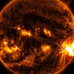


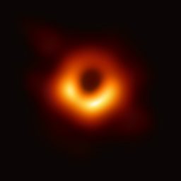



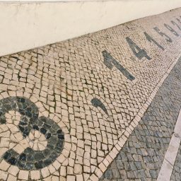


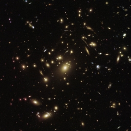


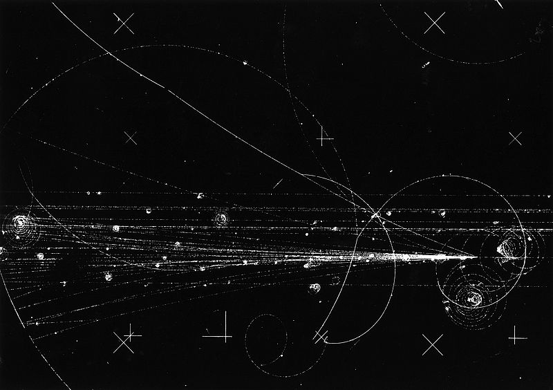




.jpg)