When the state of a subatomic particle cannot be described by a wave function without taking the state of another subatomic particle into account, we speak of quantum entanglement. It’s the special case where both particles can only be described by one and the same wave function. No longer are they separate entities nor do they have separate wave functions. The astonishing consequence is that performing a measurement on one particle has an immediate effect on the measurement of the other particle, no matter how far apart they are from each other. In this article, the second part of our mini-series on quantum entanglement, we will discuss the EPR paradox which Einstein and colleagues put forward. After that, we will discuss Bell’s Theorem which allowed physicists to test Einstein’s proposal. Was Einstein correct?

Quick summary
Firstly, let me give a quick summary of the previous post:
1. we used the property of spin as a way of distinguishing between the two entangled electrons;
2. the orientation of an electron’s spin is expressed as spin up (anticlockwise) or spin down (clockwise) along the axis of measurement;
3. you can arbitrarily choose along which axis you want to measure its spin, in three dimensions;
4. no matter which axis you choose, the result is always going to be a spin up or spin down (there is no spin-a-bit-to-the-right, for instance);
5. we are able to entangle particles in such a way that they will either always yield opposite spin or they always yield identical spin; once prepared this way, they will never deviate from this correlation when measured;
6. we used the opposite-spin entanglement in our example and we will do so again here;
7. quantum mechanics states that before measurement neither electrons have a specific spin: the wave function contains all possible measurement outcomes, in this case pertaining to both spin up and spin down (which can be characterised as having no definite spin yet)(beginfootnote)Analogously, the double-slit experiment showed that before measurement, particles don’t have a specific location yet.(endfootnote);
8. as soon as you measure one electron’s spin along a certain axis, the other electron’s spin immediately snaps to the opposite orientation along that same axis, regardless of spatial distance between the two entangled particles(beginfootnote)Or, if their entanglement were prepared in such a way that they always have identical spin, the other electron would then immediately snap to the identical spin orientation along the same axis of measurement.(endfootnote).
EPR paradox
Even though Einstein understood quantum mechanics like few others, and while accepting these predictions and results, he didn’t quite like the non-local implications brought forth by quantum entanglement. He didn’t like point 8 of the previous section. There seems to be zero time delay between influencing a particle in Amsterdam (through measuring its spin) and influencing its entangled particle in Boston. It violates a pivotal consequence of Einstein’s theory of special relativity: no signal or piece of information – anything within this universe, really – can exceed the speed light(beginfootnote)In a vacuum.(endfootnote) or else causality would not exist. In other words, if information or signals were able to travel faster than light, an effect could occur before its cause had taken place. To put it mildly, this doesn’t seem to be the universe you and I are living in.
So, Einstein, Podolsky, and Rosen (EPR) hypothesised that something else, something secretive was going on in nature – well out of sight for theoretical and experimental physicists. Quantum mechanics as it was known then had to be incomplete. Obviously, they acknowledged its successes, but when it came to quantum entanglement, they asserted something was missing in the theory of describing nature through wave functions.
To solve for the seemingly faster-than-light signal, they proposed that what really was going on was that the particles have always been in a specific state. When the electron pair were separated from each other, they have always had either spin up or spin down from the start from the moment of their creation.
Suppose, a pair of gloves were made. Like all pairs of gloves, they always were each other’s opposite with respect to ‘handedness’(beginfootnote)‘Handedness’ in this context is a form of the more generalised term chirality.(endfootnote). One has always been left-handed, the other has always been right-handed. And if the first one happened to be right-handed, then the other was left-handed. (Or else you’re holding a glove from another pair.)
Suppose, the machine which had made the pair put each glove in a separate box. We can’t see which glove went in which box until we open the box. The boxes were sent to Amsterdam and Boston. The experimental physicists then open the box in Amsterdam: it’s the right-handed one! And so, we now instantly know, the one in Boston is left-handed. No magic, no non-locality, no lightspeed-breaking shenanigans.

This is what Einstein and friends said was happening in the case of electrons. An electron pair always had specific spins to start with. It’s only in Amsterdam and Boston that we ‘open the box’ aka measure their spin. It’s only logical now that as soon as you know which spin the Amsterdam electron has, you immediately know which spin the Boston electron has.
So, said Einstein, non-locality is an illusion. It’s all just normal local laws of nature and a bit of logical thinking. For one, spin orientation is merely hidden from us and not principally uncertain. Secondly, there’s no spooky action at a distance[1], as he famously described it(beginfootnote)In German, he wrote ‘spukhafte Fernwirkung'[1].(endfootnote).
In everyday parlance, physicists call this a local version of the ‘hidden variables’ theory. ‘Hidden variables’ pertain to the stuff that we can’t see yet (such as spin orientation or other variables influencing this) because our quantum mechanical description (the wave function) is incomplete, however, they are there, they do exist – they do not not exist yet, according to the hidden variables theory.
Bell’s inequalities
Unfortunately, Albert Einstein passed away in 1955. And Niels Bohr, the other great physicist with whom he used to debate the fundamental nature of quantum mechanics passed away in 1962. In both cases too soon for them to be able to read John Stuart Bell’s 1964 paper called ‘On the Einstein Podolsky Rosen Paradox'[2]. Bell realised that Einstein’s proposal was in principle testable. It yielded a clear prediction, called Bell’s inequality.
At this point, we must note that over the years, more than one Bell’s inequalities have been put forward by physicists(beginfootnote)Besides his original inequality, there’s the much-used CHSH-inequality, for instance.(endfootnote). To explain Bell’s inequality, we will apply a version of David Mermin’s original version as mentioned in his fantastic Boojums All the Way Through: Communicating Science in a Prosaic Age[3].
Recall from point 3 before that we can measure an electron’s spin orientation along any axis. We’re going to be measuring along three axes. These axes will be at an angle of 120° relative to each other.

The first axis will be the spin orientation along the vertical axis, which we will denote with the following symbols for spin up and spin down:
$$\uparrow \downarrow$$
The spin orientations up and down will also be measured along this second axis:
$$\nwarrow \searrow$$
And the spin orientations along the third axis will be denoted by:
$$\nearrow \swarrow$$
So, imagine two entangled electrons being separated in space from each other. The usual quantum-mechanical description of each electron is that they are in a superposition of spins up and spins down for all three axes.
Except, Einstein says, no, no, not really: hidden behind the ‘veil of superposition’ they are in fact already in definite, specific spin orientations for each of the three axes. We just don’t yet know which until we measure them!
He says, the electron in Amsterdam may already be in the specific spin states as follows:
$$\left( \uparrow \searrow \swarrow \right)_A$$
So, along axis 1 it’s spin up, along axis 2 it’s spin down, and along axis 3 it’s also spin down.
Einstein continues and says that the entangled electron in Boston has to already be in the opposite states:
$$\left( \downarrow \nwarrow \nearrow \right)_B$$
And so, Einstein concludes, as soon as you actually perform a measurement in Amsterdam along the first axis, of course, you get the opposite spin in Boston. Only logical!
Bell’s insight was that if you would work out this entire argument for all possible combinations, you could actually get a prediction of a ratio of outcomes. Here’s how that goes.
First of all, if you measure along axis 1 in Amsterdam, that doesn’t mean you have to measure along that same axis in Boston. You could just choose to measure along axis 3. So, with the two examples above, your results would simply be that in Amsterdam you get spin up and in Boston you also get spin up:
$$\left( \uparrow \right)_A \text{ and } \left( \nearrow \right)_B$$
Bell then argued, if you would count the number of times you would get the combinations up-up, down-down, and of course up-down and down-up like this, you should get ratios of these combinations which should match experiment. If, however, these ratios don’t appear in the experiments, then Einstein’s hypothesis is incorrect. In that case, something entirely different is going on. The electrons were not already in a specific state, which in turn means that the non-local measurement effect in quantum entanglement does exist!
Bell’s theorem
So, let’s put them all together. Let’s first take our example above:
$$\left( \uparrow \searrow \swarrow \right)_A \text{ and } \left( \downarrow \nwarrow \nearrow \right)_B$$
If you measure along axis 1 in Amsterdam and along axis 1 in Boston you get spin up, spin down. If you measure along axis 1 in Amsterdam and along 2 in Boston, you get spin up, spin up. And so on, and so forth! We’ve put it in a little table:

Here you can see all the possible combinations of measurement outcomes along the three possible axes of the electrons in Amsterdam (A) and Boston (B). We used U for spin up and D for spin down.
Bell then says that if Einstein was correct, and the states of the spin orientations along these three axes were already there, then these are the expected outcomes.
Let’s focus on the number of UD or DU combinations, in other words, let’s focus on the number of times we find the opposite spin orientations, irrespective of the axes along which they are measured. We’ve marked them yellow.

Exactly five out nine times you will find the opposite spin directions.
Let’s check for other spin combinations. Suppose, the electron in Amsterdam is secretly in the following spin states, $\left( \downarrow \nwarrow \swarrow \right)_A$, and the electron in Boston is then the opposite, $\left( \uparrow \searrow \nearrow \right)_B$. If we count again the number of times the measurement outcome of opposite spins, we get, again, five out of nine.

Okay, I think you can imagine where this is going. We’re not going to go by all the tables, but I do want to do one more, just for fun. Suppose, the one in Amsterdam is all spin down, $\left( \downarrow \searrow \swarrow \right)_A$, and, obviously, the Boston one is its opposite, $\left( \uparrow \nwarrow \nearrow \right)_B$. In that case, we would get opposite spins in nine out of nine times.

And so, this particular Bell inequality states that the probability (P) of finding opposite spins along all three axes is at least $\frac{5}{9}$ or 55% (and at most 1 or 100%). In other words, $P(\text{opposite}) \geq \frac{5}{9}$. If this inequality were violated by experiment, the underlying theory will have been proven to be incorrect.
Experimental outcomes
Over the past thirty years, many experiments were carried out to test multiple versions of Bell’s inequality. Usually, these tests involved photons rather than electrons and pertained to measurement of polarisation rather than spin.
Freedman and Clauser did the first Bell test. They used a version of the so-called CH74 inequality[4].
The most well-known test was performed by Alain Aspect and colleagues. As Bell had originally suggested, they were able to have the two measurement devices randomly select the method of measurement before the entangled photons had arrived[5].
In all tests, all versions of Bell’s inequalities were violated. Instead, the statistical outcome was congruent with the predictions of quantum mechanics. The conclusion has to be that Einstein’s local hidden variable theory was incorrect. There is nothing local about measuring entangled particles.
In our particular inequality, the result was that the occurrence of opposite spins turned out to be exactly 50%, not 55%.
Conclusions
Let’s summarise what we have established over the course of the last two posts, including this one.
In quantum mechanics, particles which have not been measured yet don’t have a definite, specific state. Instead, they are best described by a wave function which incorporates all the possible future states it can snap into once measured.
When a particle can only be described in tandem with another particle, i.e. both particles can only be described by one and the same wave function, they are maximally quantum entangled(beginfootnote)In practice, in the real world, particles aren’t maximally entangled like the way we can prepare them in the laboratory. The world is too messy for those ‘pure states of entanglement’ to exist for any significant amount of time. There are simply too many particles around to not interact with any other particle. Every particle will invariable interact with thousands of trillions of other particles and so any previous entanglement will quickly decohere into either a very weak version of the original entanglement or simply to zero entanglement. Every interaction represents a measurement. Since our brains are too large and consist of thousands of trillions of particles, they will never be in a pure state of superposition nor entanglement. Not to mention our much larger body, which will never be in any sort of quantum state. It is statistically so unlikely that you’d have to become as old as $(10^{100})^{100}$ times the age of our current universe to witness such an event. And that number was a metaphorical one. It’s much larger.(endfootnote).
If their entanglement entails their spins will always correlate in a certain way – be it identical spins or opposite spins – a measurement on one particle, causing it to snap into one of the possible, specific, definite states, has immediate effect on the state of the other particle: it instantly snaps out of its wave function haze into a correlating, specific, definite state.
Einstein didn’t like this as this would imply some kind of information was somehow transported beyond the speed of light from one particle to the other.
He postulated that particles have always been in a specific, definite state to begin with. The only reason we don’t know which is because we haven’t measured it yet. There is no ‘snapping out of the haze’ going on.
John Bell showed that Einstein’s hypothesis can be tested. If you would perform many, many measurements of many, many maximally entangled particles, eventually, the occurrences of the variety of correlated states should show up in a certain ratio, an inequality, as it happens.
Experiments showed they do not. Instead, the ratio is exactly according to the predictions of quantum mechanics.
This demonstrated that particles indeed snap out of their haze upon measurement and not that particles had always been in a hidden but definite state.
And if that is true, then non-locality has to be true – there is no other way the other particle snaps into the correct, correlated state.
Nobody knows how this happens. Certain non-local but still hidden-variables hypotheses have been proposed. One of the more famous versions is called the ER=EPR conjecture by Juan Maldacena and Leonard Susskind. Perhaps we’ll dive into that later on.
Einstein’s aversion to this ‘particles have no definite state until measured upon’ made him utter his famous complaint, ‘God does not play dice’.
Unfortunately, he was wrong here on two occasions. God(beginfootnote)We are using the word ‘God’ in a purely metaphorical way. This does not pertain to any specific religious entity as revered by many in a variety of societies in human culture.(endfootnote) does play dice. Moreover, He throws them where we can’t see them. Even God seems to be bound by Heisenberg’s Uncertainty Principle. But that’s a subject for another bit of maths and physics.
[1] Einstein, A., Podolsky, B. and Rosen, N. (1935) “Can Quantum-Mechanical Description of Physical Reality Be Considered Complete?,” Physical Review, 47(10), pp. 777–780. doi: 10.1103/PhysRev.47.777.
[2] Bell, J. S. (1964) “On the Einstein Podolsky Rosen Paradox,” Physics Physique Fizika, 1(3), pp. 195–200. doi: 10.1103/PhysicsPhysiqueFizika.1.195.
[3] Mermin, N. D. (1990) Boojums all the way through : communicating science in a prosaic age. Cambridge England: Cambridge University Press.
[4] Fry, E. S. and Thompson, R. C. (1976) “Experimental Test of Local Hidden-Variable Theories,” Physical Review Letters, 37(8), pp. 465–468. doi: 10.1103/PhysRevLett.37.465.
[5] Aspect, A., Dalibard, J. and Roger Gérard (1982) “Experimental Test of Bell’s Inequalities Using Time-Varying Analyzers,” Physical Review Letters, 49(25), pp. 1804–1807. doi: 10.1103/PhysRevLett.49.1804.
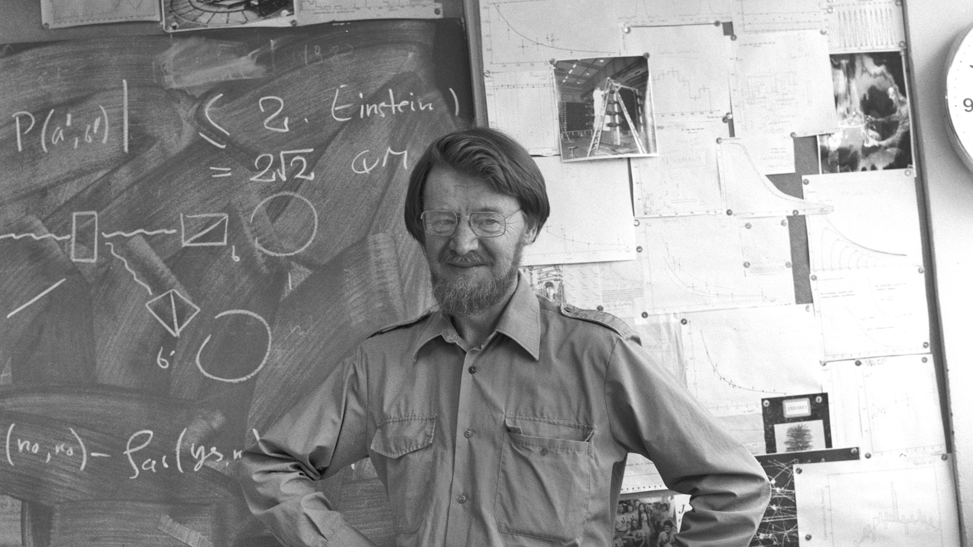
Featured image: Portrait of theoretical physicist John Bell at CERN, June 1982 (CERN, CC BY 4.0)