As is usually the case with scientific buzz words in everyday parlance, in books, in the cinema, on TV, and on the internet – like energy – the meaning of the word dimension rarely aligns with what mathematicians and physicists understand it to be. This day and age it’s rather uncommon to not have been exposed to phrases such as ‘higher’ or ‘other dimensions’. It’s likely you’ve used them yourself once or twice in your life. In this episode, we’ll explore what mathematicians and physicists mean when they talk about dimensions, and, more interestingly, the spaces they yield.
Dimensions are not Universes
In science-fiction or even everyday lingo, the word ‘dimension’ is often synonymous with entire worlds, or realms or (pocket) Universes. For instance, aliens may have come from another dimension. Or souls or ‘essences’ dwelling on a ‘higher plane of existence’ in another ‘dimension of reality’ are spoken about.
On a regular basis, portals to other dimensions are opened from which exotic forms of matter and energy are extracted to benefit either the hero or the bad guy of the story.
It’s also a favourite way to travel great distances within our reality. Just hop through a dimensional portal and out you come, back into our reality, only thousand kilometres away from where you started. Occasionally, you may also travel in time by flying through other dimensions.
And, of course, other dimensions can be summoned into our own reality or, if the story goes that they have always been present inside our reality, they can be made visible by powerful minds. This is, again, alluding to dimensions being whole separate realms within our realm.
Figure 1. Doctor Stephen Strange (Benedict Cumberbatch) is about to step into the Mirror Dimension as summoned within (or next to) our reality by his mentor, the Ancient One (Tilda Swinton), in the 2016 film Doctor Strange of the wildly popular Marvel Cinematic Universe (MCU). License note. (Click to enlarge.)
This whole section was just to let you know that what is meant by dimensions in most science-fiction stories is not what is meant in mathematics and physics. They are not realms, realities, worlds or pocket Universes. If we were to refer to realms, realities, worlds, and Universes, we would just say realms, realities, worlds, and Universes, but not dimensions.
Ordinary spaces and dimensions
So, what do mathematicians and physicists mean when they talk about dimensions?
In many cases, they pertain to the actual directions you and I are able to travel in ordinary space. I prefer to think of birds and fish as gorgeous examples of being able to travel in all directions of space all by their own.
They can fly from your left to your right and vice versa (first direction). They can fly head-on towards you and whizz by over your head and fly further behind you and vice versa (second direction). And, obviously, they can fly up from underneath you and they can keep on flying to way above your face. And vice versa (third direction).
In many cases, all three directions are oriented perpendicularly with respect to each other. To use another word, they are orthogonal. All motion can be described as some combination of moving in these three orthogonal directions, i.e. orthogonal dimensions.
In high school we have gotten all too familiar with these three dimensions. We were tortured with finding distances between vertices of a cube along the edges, the sides, and straight through the block. Of course, this is what modern gadgets and cinematography refer to when they use the term 3D, three-dimensional. In some way or form, all three orthogonal dimensions are either taken advantage of or simulated in a virtual way.
Mathematically, the capability of travelling (or ‘transporting’) along these three orthogonal directions automatically give rise to a space, a topology, of some shape or form. Ordinary space is the space you and I are born in and have grown very much accustomed to.
So, while dimensions may give rise to spaces, they are definitely not the same. Besides, while one dimension by itself technically yields a topology, a space, it’s still a one-dimensional space, meaning, no three-dimensional bodies are able to traverse this without being torn apart.
Figure 2. In ordinary space, we have three dimensions in the $x$-direction, the $y$-direction, and the $z$-direction. In high school, we were to calculate the distance between points $O$ and $F,$ for instance.
Euclid and Descartes
A very informal definition of dimensions is the number of coordinates needed to locate an object (in a space of some kind). So, on a flat surface (a plane), such as a ceiling, you need two coordinates to locate a fly. A fly can be 2 metres away from the left wall (the first direction) and 3 metres away from the back wall (the second direction, perpendicular to the first direction). Its coordinates are therefore (2,3). Hence, a plane is two-dimensional.
In ordinary, three-dimensional space, we need three coordinates to locate a fly in a room. A fly can be 2 metres away from the left wall, 3 metres away from the back wall, and 1.5 metres up from the floor. Its coordinates are therefore (2,3,1.5).
This was one of René Descartes’s great insights while lying in bed late in the afternoon or so the story goes. Hence, these numbers are called Cartesian coordinates. Descartes was pivotal to the development of what we now call the Cartesian coordinate system.
The space to which these type of coordinates belong is called Euclidean space as the great Greek mathematician Euclid was the father of Euclidean or classical geometry.
I think I can safely say that Euclid and Descartes enabled mathematics teachers to torment us with a whole slew of homework in order for us to fully explore the realm of Euclidean space in both two- and three-dimensional Cartesian coordinate systems.
Figure 3. Home of Descartes in Utrecht, the Netherlands, where he wrote parts of his famous Discours de la Méthode. The house has been demolished. Nowadays, the place looks very different. (Click on the image for a link to the original Instagram post where you can also swipe for the photo of what is looks like today. Opens a new tab.)
Space and time
In real life, besides a position in ordinary space, you also need to specify when. Getting the coordinates to be inside an office located on the corner of two streets on the 24th floor (that’s the three dimensions of ordinary space right there) just isn’t enough. You also need a time-coordinate. When are you supposed to be there?
Einstein called the fact that you’re inside an office at a certain time an event. In other words, where, in ordinary, Cartesian coordinates, we talked about some thing being somewhere, Einstein had the insight to now only start talking about events taking place in terms of space and time, space-time – using space-time coordinates.
When Einstein introduced the special theory of relativity, the German mathematician Hermann Minkowski realised this theory could also be understood geometrically in a four-dimensional space-time, where time is taken to be the fourth dimension. We now call this space Minkowski space. Note that we’re using the word ‘space’ in a broader sense: it doesn’t just encompass ordinary spatial dimensions but it now also includes a dimension of time (and, for technical reasons, isn’t Euclidean).
By the way, another word mathematicians and physicists like to use is manifold. A manifold is a topological object which can take many shapes – such as a two-dimensional plane, a three-dimensional Euclidean space, four-dimensional Minkowski space or any other space you can mathematically think of.
In Einstein’s general theory of relativity (gravity), we still work with four-dimensional space-time, except the shape of the space isn’t Minkowskian any more. The shape of the space is warped, curved, and stretched. In the best theory of gravity we have to date, we work on a so-called pseudo-Riemannian manifold, named after the great German mathematician Bernhard Riemann. The dimensions are still all the directions you can take on this manifold, i.e. the minimum amount of coordinates you need to locate an event. However, in this case, they are not necessarily oriented perpendicularly with respect to one another.
Figure 4. In the film Interstellar (2014), director Christopher Nolan featured an object which had something to do with space and time. (Click to enlarge.) If you haven’t seen the film and still intend to, do not read this footnote:(beginfootnote)Astronaut Joseph Cooper (Matthew McConaughey) finds himself in this spatial representation of space-time. All four dimensions of particular events in the past, present, and future of a room in his house, chopped up into manageable time chunks, are mapped onto an object (called a Tesseract) inside of a black hole (where the roles of space and time are reversed) through which Cooper can transport himself freely. This enables him to trickle information into the events of his choosing. In the still image above, you see many instances of the same room of his house with his daughter at different positions in time (which is the equivalent of different positions in space for Cooper).(endfootnote). License note.
Four ordinary space dimensions
Imagine a Pac-Man living on the surface of a sphere. To them, the world is flat. If they were to travel straight on – and on and on and on – eventually, they would be quite surprised to find themselves returning to the point where they started.
Figure 5. Imagine being as flat as a Pac-Man, travelling on what seems to be a flat surface. You might be surprised to find you’d eventually end up where you started. If you had no knowledge of the three-dimensional concept of a sphere, that is. We do. We know that you’d return because that’s what a sphere – or a circle, for that matter – does to your path. But what about our Universe? What if we would travel billions and billions of years in a straight line through the Universe? Would we end up where we started? Could our Universe be some kind of hypersphere(beginfootnote)Yes, technically, it’s a glome, or an n-sphere, where $n=3,$ and the space it’s embedded in is $n=1$, not a hypersphere. Apologies to the mathematicians and physicists.(endfootnote)?
We, the three-dimensional beings most of us are, see them as a little surface, a shape, because we can see them ‘from above’, from the third dimension. We can also see how they’re travelling around the surface of a sphere. They don’t know what a sphere is. They only think of flat surfaces. To us, however, it’s quite logical they would eventually return to their point of origin.
Okay, so, back to our 3D world. Imagine we travelled in a spaceship, always in a straight line through the Universe. Now imagine, after billions of years, we end up where we started: Earth. What happened? Could our Universe be some kind of sphere, only four-dimensional?
While no experiment has proven the existence of a fourth spatial dimension (let alone five or six etc.), it is a wonderfully entertaining world for the mind to ponder about.
Just to be absolutely sure: time is not the fourth dimension we’re talking about here. We were talking space – spatial dimensions. Quite often these two get confused: four-dimensional space-time is three spatial dimensions plus one time-dimension while four-dimensional space is four spatial dimensions without time.
Abstract spaces
There’s another way in which dimensions and spaces are used by mathematicians and physicists. Imagine an object having several properties at once: a position (in ordinary space), motion, direction of that motion, temperature, colour. To describe the state of this object, you need more than just four space-time coordinates. Suppose, its space-time coordinates are (0,1,1,1), in other words, it exists at time $t=0$ at position $(x=1; y=1; z=1)$.
Did we describe the state of the whole object? No, we’re still missing some key properties here. It is in motion, so, it has a speed, say 10 m/s. That speed has a direction – this is why we say it has a velocity, which is speed and direction. Let’s say its velocity $v = -10 \text{ m/s},$ in other words, it has a speed of $10 \text{ m/s}$ to the left.
Let’s say its temperature is 273.15 Kelvin, which is 0 ℃ and 32 ℉. And its colour is pure white. So, how many numbers do we need to describe the object’s state fully? Exactly, seven numbers (we count ‘white’ as a number).
The coordinates (0,1,1,1,-10,273.15,white) are said to live in phase space, an abstract space where the properties of the object form the dimensions of that space. This particular phase space is seven-dimensional. Of course, that’s impossible to imagine, but mathematically, you can work very well with it.
We gave an unusual example to emphasise that dimensions needn’t be related to spatial and temporal positions. However, usually, phase spaces are indeed used in the context of position and momentum.
Figure 6. A sample trajectory through phase space is plotted near a so-called Lorenz attractor, a solution to the Lorenz system, which Edward Lorenz developed to model atmospheric convection. The colour of the solution fades from black to blue as time progresses, and the black dot shows a particle moving along the solution in time. The three-dimensional trajectory in phase space is shown from different angles to demonstrate its structure.
Another example of an abstract space is a so-called vector space where each coordinate does not just occupy a point in that space but that point also has a direction. An example of such a space is the velocity of wind. Each point in that space does not just have a value pertaining to the speed of the air and its location in ordinary space, it has a direction too.
In the previous post, Complex numbers: an introduction, an entirely new kind of number line was introduced. All the spaces we just mentioned could very well contain complex dimensions. In fact, most of the time, they do. Especially in quantum mechanics. Complex numbers make up abstract complex vector spaces where wave functions thrive. Hilbert space is where it’s at, most of the time.
The Standard model of quantum physics is based on groups of symmetrical transformations in complex space, called SU(3) $\times$ SU(2) $\times$ U(1). The S stands for special and denotes all possible transformations in complex space except for one particular kind. U(1) refers to a one-dimensional unitary circle group in the complex plane. The numbers indicate the number of dimensions in which these transformations take place. The number of dimensions of the entire system is much higher, though! The dimensionality of the abstract complex space which follows from a symmetry group such as SU(3) is $3^2-1=8.$ As you can see, compared to street corner vernacular, dimensions are very different in scientific context.
In general, we can say that every manifold is a space. This needn’t pertain to spatial space. The minimum amount of dimensions needed to construct a path to a point on that manifold is the dimensionality of that space.
There are so many more types of mathematical spaces, they’re too many to mention. Suffice to say, while they have nothing to do with our ordinary space – our real-world one, which we dwell in – all these abstract spaces are brilliant mathematical tools enabling us to do predictive calculations pertaining to phenomena taking place in our ordinary, real-world space.
String theories
An interesting beast among all of this is string theory. If you accept the premise that an elementary particle such as an electron is actually a spatially one-dimensional string vibrating in specific ways corresponding to the collection of properties of an electron, then more dimensions are automatically needed in order to describe all the particles in this way. Strings need a sufficient amount of freedom, degrees of freedom, to vibrate in unique ways to be able to encompass the entire zoo of elementary particles and their properties.
Figure 7. The basic building blocks of the entire Universe, according to string theory. Unfortunately, while the theory is mathematically consistent, it cannot yet be (and hasn’t been) proven to be correct in this Universe.
In various versions of the string theories, a varying number of dimensions are needed. These dimensions are spatial and invisible. Since we don’t experience these dimensions, it is hypothesised that they are extremely small and curled up. They’re not stretched out like our ordinary three spatial dimensions.
Or they are so large that to us they don’t affect us in any way noticeable. Just as the curvature of Earth did not affect us when we were little as the Earth is so big compared to our movements.
Unfortunately, the theory cannot be tested yet. For now it’s purely a mathematical exercise. Although many discoveries have been made in pure mathematics, no experiment has proven string theory to be true (string theory in all its variety, and I’m including superstring theories and M-theory here even though the hierarchy is the other way around). No extra dimensions have been found yet.
There’s one honourable mention that I’d like to make. It’s the Calabi-Yau manifold, or the Calabi-Yau space. In superstring theory the manifold is hypothesised to encompass six invisible extra dimensions for the theory to work. The manifold is three-complex-dimensional or six-real-dimensional. I like it because it looks cool.
None of this is proven; we seem to be stuck in this three-dimensional space with one direction of time. And, if you ask me, it’s likely that our three-dimensional space turns out to be a side product of something quantum.
Figure 8. A Calabi-Yau manifold, named after Eugenio Calabi and Shing-Tung Yau. This is a complex space with complex dimensions. It yields applications in theoretical physics, most notably in superstring theory, where the manifold has six dimensions. Though not experimentally proven to be existing in our world, they do yield fascinating mathematical possibilities and puzzles.
Spaces and dimensions
There are so many different spaces with a variety of dimensions that you’d need a whole slew of posts to describe them all properly.
What can we take away from all of this? Dimensions are not realms. In ordinary space, they are the directions in which objects can freely be transported. That’s three for our world.
If you model time as a dimension, then we live in a four-dimensional space-time world. Except that you can’t freely move in time as there’s only one direction(beginfootnote)Time is definitely going to be a whole separate set of posts. Can’t wait.(endfootnote).
Though many had hoped to find extra spatial dimensions, the largest experiment humankind has undertaken, the Large Hadron Collider at CERN, has not found a shred of evidence for them. Instead, it delivered convincing evidence that the current Standard Model of particle physicswithout extra dimensions is still correct.
Nevertheless, to describe and predict phenomena in our Universe, it is almost always helpful to model their properties as extra dimensions. This has nothing to do with there actually being extra dimensions – this is probably where popular and esoteric culture get their inspiration from – but has everything to do with being able to do calculations in the abstract world of mathematics.
In a previous post, for example, we assumed imaginary time as an extra dimension to mathematically derive a set of equations in the special theory of relativity. It doesn’t mean imaginary time is an actual extra dimension you can dip appendages or your consciousness into.
In string theories, actual extra spatial dimensions are required for the theories to work. None of them can be tested as of yet (and none of them have been tested nor proven). It remains to be a beautiful, mathematical construct, but only mathematical.
In future posts, we will be exploring geometry, pseudo-Riemannian manifolds, symmetry groups, and Hilbert space for loads more bits of maths and physics.
Licenses
The featured image in the title and Figures 1 are still images of Marvel Studio’s Doctor Strange (2014) and Figure 4 of Interstellar (2014), all copyrighted films. It is believed that screenshots may be exhibited under the fair use provision of United States copyright law.
Figure 6. Lorenz attractor animation by Dan Quinn under CC BY-SA 3.0
In 1905, Albert Einstein published an article on moving bodies and electrodynamics. He noticed that Newton’s mechanics of moving bodies weren’t compatible with Maxwell’s equations of electromagnetism. In this article, he reconciled the two by modifying the first. These ideas and mathematical derivations became what we now know as Einstein’s special (theory of) relativity. In this post, we will describe some of its important bits. We start with two fundamental propositions. For the geeks, we will end with answering why special relativity is special.
Einstein’s postulates
His first postulate is basically that, whether or not you’re standing on a moving object, such as a ship, a train, or in your car, the same laws of physics apply. If you’re standing on a platform at the train station and you throw a ball in the air, the laws of physics ensure your ball comes down again. If you’re standing in a moving train, that ball still comes down again because the same laws of physics apply. The fact that you’re in motion doesn’t change anything to the rules of the Universe.
Einstein’s second postulate is basically that, by extension of the first one, the speed of light is the same for everyone. He recognised that Maxwell and colleagues correctly describe light as an electromagnetic disturbance propagating according to the electromagnetic laws of physics. He also recognised that the velocity of the light source plays no role in Maxwell’s equations. And so, if the first postulate is correct, then irrespective of the velocity of an observer relative to the light source, light travels at the same speed $c$ ($c$ is about 300 000 000 m/s) and nothing can go faster.
Whether you’re on the train or standing on the platform, the laws of physics are the same. The propagation of light is a law of electrodynamics not involving the velocity of its source. Hence, its velocity is the same on the train as on the platform, irrespective of its source or the train’s velocity.
Intuition works mostly, just not really
Suppose, you’re standing on a train station’s platform. A train passes at a speed of 30 metre per second. From inside the train, our friend throws a tennis ball out the window but in the direction of where the train is headed, at 2 metre per second, right at you. You catch it. At what speed does the ball hit your hand?
Intuitively, you might say, that’s 30 + 2 = 32 metre per second. This way of calculating is very useful, most of the time. Instinctively, you would simply add the train’s speed and the throwing speed together. This is how Isaac Newton(beginfootnote)And Galileo Galilei before him as this is the so-called Galilean transformation.(endfootnote) would want you to do it. And, mostly, he’s not wrong. Except, well, he is kinda.
Let’s wonder what would happen if our friend didn’t throw a ball, but, instead, switched on a pocket torch. The train still passes at 30 m/s. Light, however, flies out the torch at a speed of about 300 000 000 m/s. You lift up your hand. It ‘catches’ the light. At what speed does it hit your hand?
You might say, that’s 30 + 300 000 000 = 300 000 030 m/s. But no. That’s wrong. Remember Einstein’s second postulate? Irrespective of the motion of the observer, light always travels at 300 000 000 m/s and nothing goes faster, full stop. So, by our simple addition, we would have invented a way for light to go faster than light! We would be Nobel Prize winners, surely. Except, it doesn’t, and we’re not.
Something’s gotta give
So, if the speed of light is the same to our friend, on the moving train, as it is to us, standing on the platform (do read this again and realise how bonkers this is), then how the Helheim does the Universe achieve this? After he did some relatively simple mathematics – which a student in secondary education can do – Einstein realised that something was up with metres and seconds. He proved that what is a metre to us isn’t a metre to our friend and vice versa. Furthermore, what is a second to us isn’t a second to our friend either.
Basically, since we, on the platform, measure light to be going at 300 000 000 metre per second, and so does our friend on the train, well, that means that our understanding of what metres and seconds are is wrong.
The point
Here’s what’s happening. If two ‘things’, people, ‘objects’, or reference frames as physicists call them, move with respect to each other, weird things happen to space and time. Yes, the actual space and time. They are weird. We thought they were just there. Static. Always and everywhere the same. Two unchanging entities. Well, they’re not.
In the Dutch town of Leiden, the project Leiden Wall Formulas have scattered physics equations throughout the town centre. This is the Lorentz contraction, aptly placed alongside a train track: it describes how space (in this case, a one-dimensional length) is contracted, according to Einstein’s special relativity. Click here for Google Street View.
Suppose, we are on the train this time. We are in motion relative to our friend on the platform. Our friend then observes that space along our direction of motion becomes smaller, it contracts. They will actually measure our train to be shorter as compared to when it was standing still relative to our friend. They will also observe that our time is being stretched, i.e. our clock slows down. If one second goes by on their clock, they see only 0.9999999995… seconds have past on ours(beginfootnote)This number is a metaphor. The real time difference is too small for my calculator to show.(endfootnote).
And to us, being on the train, it’s our friend who is travelling (backwards!) relative to us, in fact, the whole world is travelling relative to us, backwards. So, indeed, we measure the world to be shorter in the opposite direction of our motion as well as their time being slowed down.
Twin paradox
Now, you might say, hold on: if both of us see each other’s clock slow down, then surely, there is no difference between our clocks. However, when we ride back to our friend, stop at the platform, and compare our clock to our friend’s clock, we do see that our clock is behind. This is the so-called twin paradox. If both can state the same thing, how do their clocks still differ in the end, causing one half of the twin (on the train) to be younger than the half who stayed behind (on the platform)?
This is due to the switching of reference frames: we were on a moving frame (the train), switched to a moving frame in the opposite direction (returning to our friend), and, lastly, switched to the platform’s frame, standing next to our friend, to compare clocks, while our friend never switched – he stayed on the platform(beginfootnote)Contrary to many popular and even introductory physics texts, this has less to do with acceleration, even though this does plays a role – without it, in the real world, one wouldn’t be able to switch reference frames. However, mathematically, acceleration isn’t necessary for solving the so-called twin paradox, switching frames is.(endfootnote). So, the situation isn’t symmetric.
Length contraction and time dilation. They’re not illusory, they’re real. Many experiments showed that space contracts and time dilates for things in motion as observed by things with a different motion.
To summarise in a slightly more mathematical way – Newton taught us that one platform metre equals one train metre and that the same is true for seconds:
1 platform metre = 1 train metre, 1 platform second = 1 train second.
Einstein, however, taught us that:
1 platform metre $\equiv \dfrac{1\text{ train metre}}{\gamma}$, 1 platform second $\equiv \dfrac{1\text{ train second}}{\gamma}$.
This $\gamma$ (Greek letter gamma) is crucial. It’s a factor necessary to make sure that the speed of light doesn’t get any faster than the speed of light, even if it’s on-board a moving train. This factor is called the Lorentz factor(beginfootnote)Named after Hendrik Lorentz. The expression for his Lorentz factor is as follows: \[ \gamma = \dfrac{1}{\sqrt{1-\dfrac{v^2}{c^2}}}, \] where $v$ is the speed of the other relative to us and $c$ is the speed of light.(endfootnote).
We never notice these things though. Usually, our speeds are way to slow for the effects of special relativity to be noticeable. Except for things that do go fast. Without Einstein’s special relativity, GPS satellites wouldn’t work(beginfootnote)Of course, we also need Einstein’s General Relativity for that, but that’s for another time.(endfootnote). Research institutes such as CERN and Fermilab also need to take special relativity in account for the high-energy, fast-flying particles.
So, our intuition (Newton) is mostly just fine though not precisely right.
What’s so special about special relativity
This is a somewhat technical question, requiring a somewhat technical answer, our apologies. Contrary to what is being said in many popular science texts, special relativity isn’t really about constant speeds as opposed to general relativity dealing with acceleration. In fact, special relativity is able to deal with acceleration. It’s just that it works fine as long as we’re assuming things exist in so-called Euclidean space, adhering to Euclidean geometry(beginfootnote)Named after Euclid.(endfootnote). However, after ample deliberation, Einstein concluded through his general relativity that we’re not living in Euclidean-geometric reality at all. We’re living in a Riemannian manifold(beginfootnote)Named after Bernhard Riemann.(endfootnote). In short, Euclidean space is a special case of the more general Riemannian manifold(beginfootnote)If we’re being precise, Hermann Minkowski developed a modified version of Euclidean space which we now call Minkowski space, while Riemannian manifold should actually be named pseudo-Riemannian manifold but many physicists simply call this Riemannian manifold anyway, perhaps because they’re not mathematicians.(endfootnote). Hence, we have special relativity as opposed to general relativity.
Featured image by StockSnap from Pixabay, modified by @kjrunia (added equations).
Today, fifty years ago, on the Sunday of 20 July 1969, at 20:17 UTC, aeronautical engineer, test pilot, and astronaut Neil Armstrong reported to the Mission Control’s CAPCOM(beginfootnote)capsule communicator(endfootnote) Charles Duke, and transmitted already historic words.
NEIL: ‘Houston, Tranquility Base here. The Eagle has landed.’
CAPCOM: ‘Roger, Twan— Tranquility, we copy you on the ground. You got a bunch of guys about to turn blue. We’re breathing again. Thanks a lot.’
Of course, ‘Twan'(beginfootnote)’Twan’ is (at least) a Dutch version of the French name ‘Toine’, usually given to males.(endfootnote) was a mistake but who cared because humanity had just achieved the greatest accomplishment thinkable.
This was and continued to be the stuff that dreams were made of. Many decisions to become a scientist and engineer were due to the hardly over-estimable inspiration the landing on the Moon brought to many of us and the next generations. We can only hope that a sufficient percentage of humanity will be allowed by society to continue to perform scientific research and explorations(beginfootnote)And that scientific data won’t be confused with opinions and/or regarded as part of the larger scheme of deception from a hidden agenda of those who really control the world. ??(endfootnote).
Here is a clip of the landing, courtesy of NASA: ‘It’s a 16mm film clip showing the final forty seconds of descent. It begins when Charlie Duke calls out sixty seconds of fuel remaining, and with the Little West Crater at the bottom of the window. The time-lapse video runs faster than real-time. Audio runs at normal, real-time speed, however.’
If you have time (three hours and two minutes), by all means, watch NASA’s restored Apollo 11 Moonwalk.
Science
While it was indeed an unprecedented achievement of courage, skill, and applied maths and science, the astronauts also carried out several scientific experiments, yielding some very interesting data on our solar system. Dr. Becky Smethurst, astrophysicist and research fellow at the University of Oxford, highlights the following five things we didn’t know before we went to the Moon, in a video on their YouTube channel:
the distance to the Moon,
the structure inside the Moon,
what the solar wind is made of,
what the Moon is made of,
how the Moon was formed.
We highly recommend subscribing to their channel with ever informative and entertaining nuggets of knowledge you both knew and didn’t know you wanted to know about that little agitation called Universe. Happy lunar anniversary! To everyone.
Screenshot of Dr. Becky’s video. Click to open their YouTube clip.
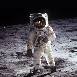
Featured image: Buzz Aldrin, made by Neil Armstrong. Courtesy of NASA.
Well-known for their central role in Einstein’s Special Relativity, the Lorentz transformations are derived from the rotation of two frames of reference in standard configuration while time is taken to be an imaginary unit of spacetime. This is rarely seen in the wild. Not many undergraduate textbooks or online texts show the details of the working. Hence, this article.
One might think this means that imaginary numbers are just a mathematical game having nothing to do with the real world. (…) It turns out that a mathematical model involving imaginary time predicts not only effects we have already observed but also effects we have not been able to measure yet nevertheless believe in for other reasons. So what is real and what is imaginary? Is the distinction just in our minds?
S. Hawking[1]
Even though there are many derivations of the Lorentz transformations to be found in textbooks, in syllabi, and online, to me, one of the most elegant remains the version Henri Poincaré once alluded to[2], which Hermann Minkowski then toyed with a bit further—to put it unreasonably mildly—in what we now call Minkowski space, but is rarely expounded in the aforementioned places.
Henri Poincaré noted that, when the time axis of the two coordinate systems has been made imaginary, i.e. the imaginary axis in the complex plane, the transformations set forth by Hendrik Lorentz pop out automatically after a rotation of two reference frames in that complex plane.
In this document, we show how this is done. We assume the reader is familiar with complex numbers.
The aim is to derive the following set of Lorentz transformations:
where $(t,x,y,z)$ and $(t’,x’,y’,z’)$ are the coordinates of an event in two frames. The primed ($’$) frame is, seen from the unprimed frame, moving with speed $v$ in the $x$-direction. The speed of light in a vacuum is denoted by $c$. As a side note, the recurring term $(\sqrt{1-v^2/c^2})^{-1}$ is called the Lorentz factor and it is usually denoted by the letter $\gamma$.
Standard configuration
Figure 1: Two frames of reference in standard configuration. A two-dimensional depiction of Hermann Minkowski’s frame M and Albert Einstein’s frame E in standard configuration: the latter moves at speed v relative to the first in the direction of x. There is no motion in either the y- or z-direction. Note that some time has passed in this diagram. At time t=0, however, their origins were equal. In other words, at temporal coordinates t=t’=0, their spatial coordinates were the same, thus x=x’=0.
Suppose, Hermann is standing still on the ground. Albert is driving his car and moves away from Hermann at speed $v$. We then have two frames of reference. There is Hermann’s frame $\mathcal{M}$ (the ground), with its origin $O$ at Hermann’s feet on the ground. And there is Albert’s frame $\mathcal{E}$ (the car), with its origin at Albert’s bottom on his chair. Their frames of reference are said to be in standard configuration as depicted by Figure 1. This means that at time $t=0$ in frame $\mathcal{M}$ where $x=0$ as well, the time $t’=0$ and position $x’=0$ in frame $\mathcal{E}$, too, and that one frame is in uniform (constant) motion relative to the other. In other words, $\mathcal{M}$ and $\mathcal{E}$ are said to be synchronised when the spacetime coordinates
\[ (t,x) = (t’,x’) = (0,0). \]
Of course, in the real world, there are four spacetime coordinates for each frame, i.e. $(t,x,y,z)$ and $(t’,x’,y’,z’)$, but to make our calculations a little bit easier, we consider the temporal coordinate $t$ (and $t’$) and spatial coordinate $x$ (and $x’$) only.
So, looking at Figure 1, we can see from Hermann’s point of view – standing in the origin $O$ of $\mathcal{M}$ – that $\mathcal{E}$’s origin $O$ moves at speed $v$ relative to the $x$-axis of $\mathcal{M}$. Speed $v$, of course, just means that $\mathcal{E}$ moves at a certain amount of units of $x$ (say, metres) per a certain amount of units of $t$ (say, seconds). This is nothing new, but it is for our derivation of the Lorentz transformations important to repeat our secondary education for a little bit:
\[ v = \frac{\Delta x}{\Delta t}, \]
in Hermann’s frame of reference $\mathcal{M}$. More or less conversely, if we want to calculate how many spatial units frame $\mathcal{E}$’s origin has moved from frame $\mathcal{M}$’s origin, we rewrite the last equation into the perhaps more familiar law of uniform motion:
\begin{equation} \Delta x = v \Delta t, \label{eq:x=vt} \end{equation}
in Hermann’s frame of reference $\mathcal{M}$.
As a side note, do realise that to Albert, his car is not moving at all; he is sitting in it. (Rather, it is the rest of the world that is moving with respect to his car and himself.) If the car were moving with respect to Albert, an accident with potentially serious consequences would be impending. So, for Albert’s sake, his speed within his own frame $\mathcal{E}$ (the car) is expressed as $v’=0$, as long as he stays put and buckled up in his chair. And so, the law of uniform motion of Albert, within his frame $\mathcal{E}$, becomes:
\[ \Delta x’ = v’ \Delta t’ = 0 \Delta t’=0. \]
Invariances
If $\mathcal{E}$ is in constant motion with respect to $\mathcal{M}$, in one direction, the $x$-direction, as expressed in Equation \eqref{eq:x=vt}, then, mathematically, we call this a geometric translation in the $x$-direction. In physics, it is called a translational motion in the $x$-direction.
Figure 2: Albert fires a photon. At time t=t’=0, Albert fires a photon P into direction x. Both the photon and Einstein’s frame E move into that same x-direction.
Suppose, at time $t=t’=0$, Albert activates his special on-board photoelectric cannon, firing exactly one photon $P$ in the $x$-direction. Figure 2 shows how the photon is travelling through the spaces of both frames of reference.
Looking at the diagram, we see that the spatial coordinates in the $y$-direction remain unchanged, $y=y’=0$, so we leave this out of our equations further on, to keep it simple. However, since $\mathcal{E}$ is moving with respect to $\mathcal{M}$ in the $x$-direction, we do know that $x\neq x’$ for $t>0$. And since we do not know for certain that $t=t’$ for $t>0$, only that $t=t’=0$, we will have to conclude that the position of $P$ differs:
Fortunately, accepting Einstein’s Voraussetzungen[3], we know that the speed of light, $c$, is the same for every frame of reference. Using Equation \eqref{eq:x=vt}, $x=vt$, and the fact that $v=c$, in this case, we can write for the distance travelled of photon $P$ – the yellow line in the diagram – in the coordinates of the respective frames of reference: \begin{align} \text{in Albert’s }\mathcal{E}\text{: }\Delta x’ &= c\Delta t’, \\ \text{in Hermann’s }\mathcal{M}\text{: }\Delta x &= c\Delta t. \end{align}
As it is possible for any coordinate system to have points which lie on the negative side of the origin of a spatial dimension such as $x$ in our case, and thus for light to travel in the negative $x$-direction, we simply square both equations to always obtain a positive value.
This is a beautiful result, because it tells us that no matter what frame of reference you happen to be in, besides $c$, Albert and Hermann agree on the quantity $(\Delta x)^2 – (c\Delta t)^2$, despite the fact that the coordinates of $P$ are not necessarily the same in every frame of reference as we saw in \eqref{eq:coordinates of P}. In other words, both $c$ and $(\Delta x)^2 – (c\Delta t)^2$ are said to be invariant.
You might wonder, what is this invariant quantity $(\Delta x)^2 – (c\Delta t)^2$, exactly? Well, this will be discussed in another post called What is a spacetime interval? And now, we might have just told you what it is. Anyway, let us move on to deriving the Lorentz transformations, and just keep in mind that $(\Delta x)^2 – (c\Delta t)^2$ is a wonderfully invariant quantity, equal in both frames of reference. Let us move on to imaginary time.
Wick rotation and imaginary time
Number sets
Figure 3: real number line. A segment of the real number line, the set R of all real numbers, which goes on to infinity on either side.
As many of us should know, Figure 3 depicts (a segment of) the real number line, that is the set $\mathbb{R}$ of all real numbers. It formed the culmination of all the previous extensions of the then-known set of numbers. Starting with the natural numbers, a set usually denoted by $\mathbb{N}$, containing all positive integers, arisen from the natural act of counting, the numeric repertoire was then extended by the notion of negative integers. Instead of just 1,2,3, we could now also count to -1,-2,-3 etc. This extension is denoted by $\mathbb{Z}$. Needless to say that $\mathbb{N}\subset\mathbb{Z}$, but we just did anyway.
Of course, some people were clever, acknowledging the need for another extension: numbers which represented ratios, better known as rational numbers, such as 1/2, 1/-3, 1/4, -1/100, in other words, quotients of two integers. These numbers would sit in-between the integers in $\mathbb{Z}$. The symbol is $\mathbb{Q}$, and it is superfluous to add that $\mathbb{N}\subset\mathbb{Z}\subset\mathbb{Q}$.
While specified on a tablet, found in Susa (Iraq) in 1936, dated as used by Babylonians around 2000 BCE, that
it wasn’t until 1761 that a proof that $\pi$ is irrational was found by Johann Heinrich Lambert[3] meaning that it could not be constructed by any ratio of integers, as were many other numbers, such as $\sqrt{2}$. And so, yet again, an extension of the existing number line was needed. This was the aforementioned line representing the set $\mathbb{R}$, or, to be precise, $\mathbb{N}\subset\mathbb{Z}\subset\mathbb{Q}\subset\mathbb{R}$.
And then, in the 16th century, people such as rivals Tartaglia and Cardano independently recognised that solutions to cubic equations sometimes required the manipulation of square roots of negative numbers, such as $\sqrt{-1}$. Later, Bombelli developed proper operations such as addition and subtraction. A whole slew of subsequent mathematicians then developed over several decennia what is now known as the complex plane or gaussian plane[5], representing the set $\mathbb{C}$, extending the real number line with an imaginary axis with multiples of the imaginary unit $i=\sqrt{-1}$. (It is, obviously, the solution to the quadratic $x^2+1=0$.) We realise mentioning that $\mathbb{N}\subset\mathbb{Z}\subset\mathbb{Q}\subset\mathbb{R}\subset\mathbb{C}$ is utterly redundant at this point.
Translation and rotation
Figure 4: Number sets. Every consecutive number set is an extension of the previous one. We can move from a simpler set to a more complex one, for instance, by simply multiplying our current position by a number only present in the more complex set. Although it seems like we are tumbling from one set to another, we are really just ‘sliding left or right’, one-dimensionally, on the number line of the more complex set. This sliding is called a translation. Note: the amount of ticks in Q is much larger, but for obvious reasons of legibility, we only ticked every 1/2-ratio.
Let us have another look at the natural number line of $\mathbb{N}$. If we would want to convert the number 1 to a number that could not exist in $\mathbb{N}$ but could exist on the integer number line of $\mathbb{Z}$, let us then simply multiply the natural number 1 with a number from $\mathbb{Z}$, the negative integer $-1$. Since $1\times-1=-1$, we have transitioned from $\mathbb{N}$ to $\mathbb{Z}$. We ‘slid’ from 1 to $-1$, albeit in a different number set, which, mathematically, is the same as a translation by $-2$. This is easily expressed as starting from position 1, adding $-2$, and ending up at position $-1$ on the number line of, at least, $\mathbb{Z}$ (but not $\mathbb{N}$): $1+-2=-1$. Figure 4a aims to depict this.
We can do the same with moving from position $-1$ in $\mathbb{Z}$ to a number not in $\mathbb{N}$, nor in $\mathbb{Z}$, but at least in $\mathbb{Q}$ by simply multiplying by a fraction, such as $-1/2$, which is also a number not in $\mathbb{N}$, nor in $\mathbb{Z}$. This is, again, actually a translation, though now by adding $3/2$: $-1+3/2=1/2$. Figure 4b aims to depict this.
Similarly, transforming from position 1 in $\mathbb{Q}$ to $\mathbb{R}$, we multiply by, for instance, $\sqrt{2}$, which exists in $\mathbb{R}$ but not in $\mathbb{Q}$, and so, the result, $1\times\sqrt{2}=\sqrt{2}$ is in at least $\mathbb{R}$ but not in $\mathbb{Q}$, nor in $\mathbb{Z}$, nor in $\mathbb{N}$. The result is also a translation of $1+(\sqrt{2}-1)=\sqrt(2)$ in $\mathbb{R}$. Figure 4c aims to depict this.
Figure 5: Wick rotation of 1 and real time. Compared to the increasing complexity of the number lines in Figure 4, this one is the most complex so far. Two Wick rotations into the complex (number) plane C, where (a) the Re-axis is the real number line of the set R and the Im-axis is the imaginary unit line of the set C. Note that a complex number consists of both: a real part and an imaginary part. For instance, the complex number z is written in the form z = a + bi, with i = √-1. The real part of z is Re(z) = a, and the imaginary part Im(z) = b. And so, z = 1 + i, z = 1/2 + 3i, z = 3, are all complex numbers, where the latter has an imaginary part of Im(z) = 0, which we simply leave out as 0i = 0. A complex number is thus two-dimensional, embedded in a plane with a real axis and an imaginary axis. (b) Wick-rotating all real numbers on the time axis to the imaginary axis, transforms real time into imaginary time.
Note that, so far, the transformation of 1 or another number has involved a simple ‘sliding’ motion on the number lines, that is, one-dimensionally. Every time a new kind of number was introduced – the negative integers, ratios, and, lastly, the real numbers – a new set of numbers was created, and the number line evolved from discrete ($\mathbb{N}$) to a line continuum $\mathbb{R}$. The question is, what would be the next extension and what would it look like?
As stated earlier, in the 16th century it became clear that a new type of number was necessary to solve a slew of quadratic equations. Owing to people such as Wallis, Wessel, Argand, Buée, Mourey, Warren, Français, Bellavitis, Gauss, and Euler[5][6], the idea to extend the real number line of $\mathbb{R}$ with an imaginary, perpendicular number line came to fruition. This created the so-called complex (geometric) plane, sometimes called the $z$-plane, Gauss plane or Argand plane. It is important to note that transforming a real number in $\mathbb{R}$ to a complex number in $\mathbb{C}$ involves not a translation but a rotation. Multiplying a real number in $\mathbb{R}$, say 1, by a number that only exists in $\mathbb{C}$, say $i$, is the same as geometrically rotating our position 1 on the real axes by $\pi/2$ onto a position $i$ on the imaginary axis as is depicted in Figure 5a.
What if we did this with the entire real time axis in a space-time diagram as shown in Figure 5b? Every element of real time $t$ is multiplied by $i$. In other words, every part is rotated in the complex plane to become an entire imaginary axis of time $it$. This procedure is called a Wick rotation, named after theoretical physicist Gian Carlo Wick, who described such a procedure to solve problems in quantum and statistical mechanics[7].
This seems promising and is what Henri Poincaré alluded to fifty years earlier. Before we continue, we have to do one other little thing. It has something to do with units of measurement.
Minkowski diagrams
Figure 6: The distance-time-diagram we all grew up with. The independent variable time t as the x-axis, and the dependent variable distance, x, as the y-axis. Four particles are travelling through time and (one-dimensional) space, each with its own distance function of time, that is, each with its own speed. Note that P travels the most amount of distance over the same period, in other words, it is the fastest. Note that S travels exactly zero distance in that same amount of time.
We all grew up learning to read and use a type of diagram as depicted in Figure 6 during our physics classes. Time is put on the $x$-axis and distance $x$ is put on the $y$-axis. Somewhat confusingly, at first, as one might have gotten accustomed to using values of $x$ on the $x$-axis during the maths lessons. Of course, one learns that it is less about the names of variables and axes, rather, it is a matter of which is the independent and which is the dependent variable. The independent one, in this case, time $t$ (time flies, whether we want to or not), is then laid out over the axis called $x$ (which has not much to do with the variable named $x$), and the dependent one, a variable which happened to be named $x$, is projected onto the $y$-axis.
In this diagram, we see four particles. The fastest, $P$, is moving away in the $x$-direction (which is up, but not necessarily up into the sky, do realise that!) covering more units of $x$ than the other three after the same time $t_1$ has passed. This is why it has a steeper slope. The slowest one is the one that is not moving at all, the stationary particle $S$. It is moving in time, which is why it exists at time $t_1$, but, spatially, it does not exist at a certain amount of units of $x$ away from the origin. In fact, it exists in exactly the same place, the origin.
Figure 7: t–x-diagram. A physicist’s diagram, where distance in space, x, is projected on the x-axis and distance in time t is projected on the y-axis. Note that the faster a particle travels, the smaller the angle of its ‘line’ through space and time with the x-axis. If the particle is stationary, it only ‘travels’ through time and the angle with the x-axis is maximised at π/2. In other words, it just goes straight up.
Well, get yourself out of the habit: turns out that professional physicists like to flip the axes when it comes to time. In other words, they project the distance variable $x$ onto the $x$-axis, while the time variable $t$ almost invariably gets to be projected onto the $y$-axis. Yes, you heard it correctly. Time goes up in a physicist’s diagram. The esteemed professor Leonard Susskind, a theoretical physicist at Stanford University, even postulated, in part jokingly, during a lecture on the principle of least action that physicists are the only type of people who do this(beginfootnote)See, for instance, https://youtu.be/3apIZCpmdls?t=1447(endfootnote). And so, we flipped our diagram as you can see in Figure 7.
Speaking of units, usually, time is measured in seconds and distance in metres. Usually. Though, remember when you went to visit those new friends of your parents and that one of the first things they assured their hosts is that their hometown was actually not that distant and that it was just ‘a two-hour drive’? Distance, while usually measured in kilometres between two places, is now expressed in units of time. Assuming that people legally drive – from door to door – at an average speed of $100\text{ km/h}$, the distance will be around 200 km.
Why do people like to express distance in terms of units of time sometimes? Well, in some cases, people aren’t interested in the exact amount of kilometres, but rather tend to focus on how much of our valuable time a certain activity consumes, hence, an answer in units of time makes sense.
Astrophysicists do another interesting distance-as-time conversion when it comes to distances between galaxies, for instance. They work with visible light reaching their telescopes, and other types of radiation. Moreover, the distances they work with are ridiculously large, especially when expressed in kilometres. So, they work with light-years, which sounds like a unit of time, but denotes a certain distance. One light-year is the distance light travels in one Julian year, which is $365.25$ days. Light travels at a speed of $c=299792458\text{ ms}^{-1}$ in the vacuum. To calculate the number of seconds in a Julian year, we multiply the number of seconds in one minute times the number of minutes in one hour times the number of hours in one day times the number of days in one Julian year:
Using Equation \eqref{eq:x=vt} to calculate distance $x$ light travels in one Julian year, we get
\begin{align} x &= vt \text{, and because }v=c\text{, we write:} \\ x &= ct,\label{eq:x=ct} \\ &= 299792458\text{ ms}^{-1} \times 31557600\text{ s} \\ &= 9460730472580800\text{ m}, \\ &= 9460730472580.800\text{ km}. \end{align}
Since light travels this ridiculously large number of kilometres, it makes perfect sense for astrophysicists to use this fact to express the distance of stars and galaxies. This way, the nearest major galaxy, Andromeda, is only about $2.5$ light-years away. This is obviously more practical than $23651826181452\text{ km}$.
So, about describing distance in terms of units of time, we learnt that
in the case of a ‘normal scale’ distance such as between two towns, expressing a spatial distance in units of time makes it easier to compare with the amount of time one wishes to spend on travelling – it becomes like comparing time with time;
in the case of larger scale distances such as between two galaxies, expressing a spatial distance in light-units of time makes it easier to handle the impractically large numbers of the original units.
Let us go back at our diagram in Figure 7 again. The units of both axes are not the same. The $x$-axis is the distance, which is expressed in spatial units, such as metres. The $y$-axis is the time, expressed in temporal units, such as seconds. It is hard to compare the two: the units are not the same. Also, as particle physicists are usually dealing with extremely fast particles, near the speed of light, it is impractical to be using the standard units of time. So, physicists have devised a solution to both problems. Number one: what if we expressed time in units of distance? So, that is the other way around: not distance in units of time, but time in units of distance.
To do that, we simply use the formula as expressed in Equation \eqref{eq:x=ct}: $x=ct$. In other words, if we multiply time $t$ with the speed of light $c$, we get a distance. A little analysis of units checks out. If we multiply the units of the speed of light with the unit of time, we get a unit of distance:
Figure 8: ct. (a) The time axis is multiplied by c, so it is easier to compare time with space, i.e. time is expressed in units of distance. (b) We set c = 1 so that the so-called world line of any particle travelling at exactly the speed of light is always at an angle of π/4 with the x-axis. Or 45°, if you are into that sort of thing.
This does not mean we magically, qualitatively, or even hypothetically transformed the time dimension into a space dimension, even though this would be a perfect device for a cool work of science-fiction, but it does mean that we now express time in units of distance. And so, we label the $y$-axis with $ct$ as is shown in Figure 8.
Now, to tackle the second problem, where physicists work with particles whose motions approach the speed of light at distance scales smaller than an electron in the vicinity of black holes with forces greater than you would ever encounter, it is impractical to work with the ordinary distance and time units. Furthermore, they prefer to choose the units of $ct$ and $x$ such, that a ‘line’ of a photon, e.g. light, travelling through space and time, is always depicted at an angle of $\pi/4$ or $45^\circ$ with the $x$-axis. To do so, they set the speed of light to 1. So, $c=1$. What you get is a diagram as shown in Figure 8(b). Particle $P$ is a photon, thus travelling at the speed of light. So, its ‘line’ is at the exact angle of $\pi/4$ with both the $x$- and $y$-axis, i.e. the $x$ and $ct$, respectively. All the other particles thus travel at a certain ratio of $c$, i.e. a certain ratio of 1.
All this should tell you enough to figure out how fast a particle would be going if its ‘line’ would be drawn underneath that of $P$, i.e. at an angle smaller than $\pi/4$. And even though you should also be able to figure out if this is at all possible, we will tell you now that this is not possible.
By the way, the term ‘line’, which we use to describe the path a particle takes through space and time in our diagrams, is called a ‘world line’ as Hermann Minkowski would have wanted us to. And the diagrams of Figures ref7 and 8 are called Minkowski diagrams. They are also called spacetime diagrams, although there is a subtle difference: Minkowski diagrams are the subset of two-dimensional diagrams within the larger set of spacetime diagrams, which contains the 3D versions, and 4D, even.
Wick rotation revisited
Figure 9: from it to ict. (a) The Wick rotation of the real time axis ct to the imaginary time axis ict. We projected the coordinate system of Figure 8 onto ‘the floor’ to have the ct-axis then rotated to the imaginary ict-axis by multiplication by the imaginary unit i. (b) Consequently, the world line of P gets rotated onto the imaginary plane as well.
We are almost ready to derive the Lorentz transformations. The only thing we have to do, is Wick rotate the (real) time axis into the imaginary time axis, i.e. we rotate the $ct$-axis of Figure 8. So, we do as we did in the previous section Number sets: we multiply by the imaginary unit $i$ from the number set $\mathbb{C}$, thereby rotating the time axis of $\mathbb{R}$ into the complex plane $\mathbb{C}$ to become an imaginary axis of time.
Figure 9 offers a geometric representation of the whole operation. We projected our original coordinate system of Figure 8 onto ‘the floor’, so to speak. We left out particles $Q$, $R$, and $S$ to keep it legible. Wick-rotating the real time axis $ct$ by multiplying by the imaginary unit $i$ then yields the imaginary time axis $ict$. Automatically, the world line of $P$ rotates along into the complex plane. Note, that the spacetime coordinates of $P$ have changed a few times in this section. They were $(x_P,t_1)$, then they became $(x_P,ct_1)$, and have ended up to become $(x_P,ict_1)$. Just the way we like it.
Deriving the Lorentz transformations
Invariant world line in the complex plane
Figure 10: Wick-rotated M and E. Hermann’s M and Albert’s E frames of reference rotated at an angle θ relative to each other in the complex plane about their origin. We put a little square with sides marked I and II to aid us in our trigonometric calculations.
To end up with the Lorentz transformations as formulated in Equations \eqref{eq:Lorentz t-prime} and \eqref{eq:Lorentz x-prime} by rotating two frames of reference relative to each other in the complex plane – with an imaginary time axis – we refer to Figure 10.
In both frames, those of Hermann and Albert, a photon $P$ travels at speed $c$. By the second postulate of Einstein’s Special Relativity[3], we know that, somehow, the value for $c$, which is chosen to be 1 in our case, is the same in both frames of reference, even though one moves relative to the other, meaning the coordinates between the frames are unequal. In Figure 2, this is represented by $v$. In Figure 10, this is represented by an angle $\theta$.
We see that the coordinates of $P$ in $\mathcal{M}$ are $(\Delta x, ic\Delta t)$. In $\mathcal{E}$, they are $(\Delta x’, ic\Delta t’)$. They are related to each other by some proportion of angle $\theta$. Before we find that relation, we repeat our finding regarding Equation \eqref{eq:interval} in the section Invariances: the quantity $(\Delta x)^2 – (c\Delta t)^2$ is invariant. In our case, it is the interval $OP$ that is invariant, despite the fact that $P$ has different coordinates. In other words, geometrically, both $\mathcal{M}$ and $\mathcal{E}$ agree on the length of the yellow world line as you can see in Figure 10. We should proceed to show this.
Let us first write down the expressions for the invariant yellow world line $OP$ in both frames of reference:
\begin{equation} \Delta x^2 – c^2\Delta t^2 = (\Delta x’)^2 – c^2(\Delta t’)^2.\label{eq:interval in the complex plane} \end{equation}
This is the result we wanted. Whether it is with imaginary time or with real time, the quantity $\Delta x^2 – c^2\Delta t^2$ remains invariant. (Recall that $i^2=(sqrt{-1})^2=-1$.) Even in the complex plane, $\mathcal{M}$ and $\mathcal{E}$ agree on the magnitude of this quantity.
Coordinates in terms of the other coordinates
Let us now express the coordinates of $P$ in $\mathcal{E}$, i.e. $(\Delta x’,ic\Delta t’)$, in terms of angle $\theta$ and the coordinates of $P$ in $\mathcal{M}$, i.e. $(\Delta x,ic\Delta t)$. Firstly, we deduce an expression for $\Delta x’$ using Figure 10:
Lastly, as we want to find the relation between $\theta$ in the complex plane and $v$ in real spacetime, we forget $P$ for a moment and now write the expression for Albert himself, sitting in $O’$ of his frame $\mathcal{E}$ in terms of the coordinates of Hermann’s frame $\mathcal{M}$. In other words, how does Hermann see Albert move? Since Albert is not moving in his own frame $\mathcal{E}$, as we said earlier, after a certain amount of time $ic\Delta t$, his $\Delta x’=0$. So, by Equation \eqref{eq:delta x prime}, we write
To recapitulate, we have now obtained Equations \eqref{eq:delta x prime}, \eqref{eq:icdelta t prime}, which express the coordinates of $P$ in $\mathcal{E}$ in terms of angle $\theta$ and the coordinates of $\mathcal{M}$. Lastly, we obtained relation \eqref{eq:tan \theta} between angle $\theta$ and speed $v$ of Albert’s frame $\mathcal{E}$ as seen by Hermann in his frame $\mathcal{M}$. So, to restate, we obtained the following transformations:
Figure 11: Triangle tan θ. The geometric representation of Equation 9: an imaginary triangle with an imaginary slope tan θ, where Γ is the hypotenuse. Note that sin θ = (iv/c)/Γ and cos θ = 1/Γ.
The Lorentz transformations
Note that, algebraically, it is possible to write Equation \eqref{eq:tan \theta} as
which, geometrically, looks like 11. Note that $\sin\theta=(\mathrm{iv/c})/\Gamma$ and $\cos\theta=1/\Gamma$, so all we have to do now, is figure out what $\Gamma$ is. Using, again, the Pythagorean theorem:
Since in our configuration the differences are calculated from the origin, we can leave out the $\Delta$-sign, using just the coordinates, and so we obtain
And so, leaving out the $\Delta$-sign, using just the coordinates, we obtain \begin{equation} t’ = \frac{t-vx/c^2}{\sqrt{1-v^2/c^2}}, \end{equation}
which is, indeed, Equation \eqref{eq:Lorentz t-prime}.
It is important to note that, while not unusual to leave out the $\Delta$-sign, formally, it is incorrect: in Special Relativity there is no preferred (fixed) origin, hence, it is always about differences.
Lastly, we reiterate that the term $1/\sqrt{1-v^2/c^2}$ is often written as $\gamma$ and is called the Lorentz factor. Also, in some texts, the term $v/c$ is replaced by symbol $\beta$, yielding the following equivalent expressions of the Lorentz transformations:
\begin{align} ct’ &= \gamma(ct-\beta x), \\ x’ &= \gamma(x-\beta ct), \\ y’ &= y, \\ z’ &= z. \end{align}
Thanks to the imagination of many mathematicians and physicists before us, our ability to investigate, analyse, and calculate has become as supple and malleable as is, indeed, the fabric of the cosmos.
[1] Hawking, S. (2001) The universe in a nutshell. New York: Bantam Books. [2] Walter, S. (2014) Poincaré on clocks in motion. Amsterdam, Ne. [3] Einstein, A. (1905) “Zur Elektrodynamik Bewegter Körper,” Annalen der Physik, 322(10), pp. 891–921. doi: 10.1002/andp.19053221004. [4] Bailey, D. H. and Borwein, J. M. (2016) Pi : the next generation : a sourcebook on the recent history of pi and its computation. Switzerland: Springer. doi: 10.1007/978-3-319-32377-0. [5] Cooke, R. (2005) The history of mathematics : a brief course. 2nd edn. New York, N.Y.: Wiley. [6] Caparrini S. (2006) On the Common Origin of Some of the Works on the Geometrical Interpretation of Complex Numbers. In: Williams K. (eds) Two Cultures. Birkhäuser Basel, pp. 139-151. [7] Wick, G.C. (1954) Properties of Bethe-Salpeter Wave Functions. Physical Review, 96(4), pp. 1124-1134.