In this post, we will derive an expression for the normal force on a uniform mass which is in planar non-uniform circular motion using polar coordinates. Finding this expression is enormously useful to calculate under which circumstances a mass would be slung off its orbital path. Of course, there are numerous situations for which we should be able find the normal force. Here, we will look at a system as shown in Figure 1. Sometimes, obtaining an expression in terms of the variables given is not straightforward. You will find a useful trick in step 7 to arrive at an expression in terms of a simple $\theta$ instead of its secondary-order derivative $\ddot\theta$ which we initially obtain.
We will apply Newton’s notation (the dot notation) whenever possible as this is the most compact form. For instance, if $\mathbf{x}$ is a vector, then its first-order and its second-order derivative with respect to time $t$ are denoted by
\[ \dot{\mathbf{x}}\text{ and }\ddot{\mathbf{x}}, \]
respectively. Where needed, in order to state explicitly that we are dealing with a time-derivative and to help in solving a time-integral for example, we will use Leibniz’s notation, i.e.
\[ \frac{\text{d}\mathbf{x}}{\text{d}t}\text{ and }\frac{\text{d}^2\mathbf{x}}{\text{d}t^2}. \]
Assignment
Look at the system as sketched in Figure 1. Imagine we stand in front of this system. Mass $m$ is attached to a model string. At $t=0$, it rests at level with the centre of the cylinder with radius $R$ with the string draped over the top. A constant force $\mathbf{P}$ pulls the string downwards. At a later time $t$, mass $m$ has slid over the top with a coefficient of friction $\mu$. Let $\theta$ denote the angle between its initial and its current position, subtended at the centre of the cylinder. Calculate the normal force on $m$, and, hence, proof that the radius of the cylinder is irrelevant.
Figure 1. The system
Step 1. Force diagrams and unit vectors
It is essential to draw force diagrams and unit vectors to define the acting forces and parameters. We choose the unit vectors to be the radial and the tangential vectors. This makes calculating most forces a lot easier. This is done in Figure 2.
Figure 2. Force diagram and unit vectors at time $t>0$
We identify the following forces on $m$:
$\mathbf{P}$ is the vector denoting the constant force pulling the model string,
$\mathbf{N}$ is the vector denoting the normal force acted on $m$ by the cylinder,
$\mathbf{F}$ is the vector denoting the frictional force,
$\mathbf{W}$ is the vector denoting the weight of $m$ as a result of the gravitational field of whatever planet the system is located,
$\mathbf{e}_r$ is the radial unit vector,
$\mathbf{e}_\theta$ is the tangential unit vector.
Step 2. Apply Newton’s second law
As this is a dynamical system, where $m$ is in non-uniform circular motion, we apply Newton’s second law, more specifically in the following form:
where $\ddot{\mathbf{r}}$ is the rate of change of the rate of change over time, that is, the second time-derivative of the displacement vector $\mathbf{r}$ of mass $m$. We can now easily identify the constituents of the vector sum as we did that already in Step 1. And so, equation (1) becomes
Step 3. Rewrite the forces in terms of their magnitudes and unit vectors
As pulling force $\mathbf{P}$ with magnitude $|\mathbf{P}|$ acts in the direction of tangential unit vector $\mathbf{e}_\theta$, we can write for $\mathbf{P}$:
Friction $\mathbf{F}$ is in the opposite direction of the tangential unit vector $\mathbf{e}_\theta$, so, we need to place a minus-sign in its expression. Furthermore, as (dry) friction is usually modelled by the product of the coefficient of friction and the magnitude of the normal force, we can write:
Lastly, weight is the force due to gravity, $|\mathbf{W}|=mg$, where $g$ is the gravitational constant. However, we need to express this force in terms of its components. In this case, those components are directed parallel to the radial and tangential unit vectors. As the latter are pointed (partly) upwards, as opposed to the downwards-pointing weight, we already know that both its components carry a minus-sign, i.e. $(-\mathbf{e}_r)$ and $(-\mathbf{e}_\theta)$. What remains, is the correct expression for the magnitude of the weight in terms of its respective unit vectors.
To clearly show how we get an expression for $\mathbf{W}$ in terms of its components along the directions of $\mathbf{e}_r$ and $\mathbf{e}_\theta$, have a look at Figure 3.
Figure 3. Finding the components of $\mathbf{W}$
What you see is just the weight vector $\mathbf{W}$ from our force diagram in Figure 2, including the radial and tangential unit vectors $\mathbf{e}_r$ and $\mathbf{e}_\theta$. For visual clarity, we subtended them on mass $m$. Also added are the two component vectors in the opposite direction of the unit vectors for which we need to find expressions.
Let component vector $\mathbf{v}_r = a(-\mathbf{e}_r)$ and component vector $\mathbf{v}_\theta = b(-\mathbf{e}_\theta)$, where $a$ and $b$ are some magnitude value such that the vector sum of $\mathbf{v}_r$ and $\mathbf{v}_\theta$ equals $\mathbf{W}$. In other words,
To find the values of the magnitude of $a$ and $b$, we use the fact that the magnitude $|\mathbf{W}| = mg$. So, using high school trigonometry, we deduce that
\begin{align} a &= mg\sin\theta, \\ b &= mg\cos\theta. \end{align}
Now, we can write $\mathbf{W}$ in terms of its components by substituting equations (7) and (8) into (6):
We can now resolve equation (12) into its radial and tangential components.
\begin{align} \mathbf{e}_r &: -mR\dot{\theta}^2 = N – mg\sin\theta, \\ \mathbf{e}_\theta &: mR\ddot{\theta} = P – \mu N – mg\cos\theta. \end{align}
Step 6. Write down the equation of motion (in polar coordinates)
Rearranging equation (14), we can write down the second-order differential equation of motion:
\begin{equation} \ddot{\theta} = \frac{P – \mu N – mg\cos\theta}{mR}. \end{equation}
While we could have solved equation (14) for $N$, this would still leave us with the second time-derivative of $\theta$. Instead, we want an expression of $N$ in terms of a simple $\theta$. This means that we need to get rid of $\ddot{\theta}$ in some way. It is not immediately clear how equation (14) or (15) should be operated on to achieve this. However, here is a neat trick.
Step 7. The trick
Have a look at the following equation where we apply the chain rule:
So, if we substitute equation (15) into (16), we get
\begin{equation} \frac{\text{d}\dot{\theta}^2}{\text{d}t} = 2\dot{\theta}\left(\frac{P – \mu N – mg\cos\theta}{mR}\right). \end{equation}
If we now integrate both sides with respect to time, we get
\begin{align} \int \frac{\text{d}\dot{\theta}^2}{\text{d}t}\text{d}t &= \int 2\dot{\theta}\left(\frac{P – \mu N – mg\cos\theta}{mR}\right)\text{d}t, \nonumber \\ \dot{\theta}^2 + A &= 2 \int \frac{\text{d}\theta}{\text{d}t}\left(\frac{P – \mu N – mg\cos\theta}{mR}\right)\text{d}t, \nonumber \\ &\text{where $A$ is an arbitrary constant}, \nonumber \\ \dot{\theta}^2 + A &= 2 \int \left(\frac{P – \mu N – mg\cos\theta}{mR}\right)\text{d}\theta, \nonumber \\ \dot{\theta}^2 + A &= \frac{2}{mR} \int (P – \mu N – mg\cos\theta)\,\text{d}\theta, \nonumber \\ \dot{\theta}^2 + A &= \frac{2}{mR} \left( P\int 1\,\text{d}\theta – \mu N\int 1\,\text{d}\theta – mg\int \cos\theta\,\text{d}\theta\right), \nonumber \\ \dot{\theta}^2 + A &= \frac{2P\theta}{mR} – \frac{2\mu N\theta}{mR} – \frac{2mg\sin\theta}{mR} + B, \nonumber \\ &\text{where $B$ is an arbitrary constant}, \nonumber \\ \dot{\theta}^2 &= \frac{2P\theta}{mR} – \frac{2\mu N\theta}{mR} – \frac{2g\sin\theta}{R} + B – A, \nonumber \\ \dot{\theta}^2 &= \frac{2P\theta}{mR} – \frac{2\mu N\theta}{mR} – \frac{2g\sin\theta}{R} + C, \\ &\text{where $C=B-A$} \nonumber. \end{align}
Solving the initial condition problem to find $C$, we use the fact that at $t=0$, angle $\theta = 0$, thus $\dot{\theta} = \ddot{\theta} = 0$. This renders $C = 0$ in equation (18), and so, we have
Note, we now have obtained an expression for $\dot{\theta}^2$ which already appeared in equation (13). We can, therefore, substitute equation (19) in (13), and we obtain:
So, now we have an expression of $N$ in terms of the gravitational constant $g$, the variables $m$, $\mu$, and $P$, and the more reasonable $\theta$ instead of $\dot\theta^2$.
And so, if we want to calculate when a mass would be slung out of its orbital path, we write $N = 0$ as this means, in physical terms, that the mass isn’t resting on the cylinder anymore (since it doesn’t exert a normal force on the mass). In other words, find the roots of equation (21) to find the one unknown variable. Note, $R$ does not play a role. Of course, bear in mind that $m$ is a point mass.
Even though the well-known Archimedes has derived the formula for the inside of a sphere long before we were born, its derivation obtained through the use of spherical coordinates and a volume integral is not often seen in undergraduate textbooks.
In this post, we will derive the following formula for the volume of a ball:
\begin{equation} V = \frac{4}{3}\pi r^3, \end{equation}
where $r$ is the radius.
Note the use of the word ball as opposed to sphere; the latter denotes the infinitely thin shell, or, surface, of a perfectly round geometrical object in three-dimensional space. A surface has no volume, hence, we prefer to refer to it as a ball.
This could be seen as a second-year university-level post.
Spherical coordinates
The volume of a cuboid $\delta V$ with length $a$, width $b$, height $c$ is given by $\delta V = a \times b \times c$.
Figure 1: A volume element of a ball
In Figure 1, you see a sketch of a volume element of a ball. Although its edges are curved, to calculate its volume, here too, we can use
\begin{equation} \delta V \approx a \times b \times c, \end{equation}
even though it is only an approximation.
To use spherical coordinates, we can define $a$, $b$, and $c$ as follows: \begin{align} a &= PQ\delta\phi = r\sin\theta \, \delta\phi, \\ b &= r\delta\theta, \\ c &= \delta r. \end{align}
Note that the relation becomes more precise when $\delta\phi$, $\delta\theta$, and $\delta r$ tend to zero. So, we can now write the volume integral for our ball $B$ as follows:
Figure 2: To integrate over the infinite number of points (inside and on the surface) of a ball, one angle varies from $0$ to $2\pi$, which is $\phi$, in this case. Angle $\theta$ only needs to vary half of that as a ball is rotationally symmetric. Of course, bound by radius $r$.
To set the upper and lower bounds for our integrals, we note that a ball has rotational symmetry about the $z$-axis (besides infinitely many others through the centre too). We will exploit this. We refer to Figure 2.
Firstly, to integrate over infinitely many points between $0$ and $r$, the lower bound is $0$ and the upper bound is $r$:
as we will proceed to, thirdly, rotate this plane, as it were, about the $z$-axis to integrate over infinitely many planes about said axis, which complete the shape of our ball. Hence, $\phi$ varies between $0$ and $2\pi$.
We will focus on a few simple problems where we will manipulate the equations for relativistic energy and momentum.
This could be seen as a second-year university-level post.
Einstein had shown that the Lorentz transformations were the correct way to switch between the coordinate systems of different frames of reference [1]. He also taught us that Newton’s laws weren’t at all proper relativistic laws. For instance, Newtonian momentum $ \mathbf{p} = m \mathbf{v} $, and energy $ E = mv^2 / 2 $ were not at all accurate at speeds approaching that of light.
Instead, we have all come to learn that the relativistic momentum is written as
Prove, for a particle travelling at $ c $, that the magnitude of the relativistic energy is given by $ E = pc $.
Show that the energy-momentum relation for a particle with any mass $ m $ travelling at any speed $ v $ is correct and do mind it is not the famous $ E = mc^2 $ we are referring to. Use the correct one, if you please.
Given that the mass of a proton is $ m_p $, calculate its exact speed when its relativistic translational kinetic energy (which is the relativistic total energy minus its relativistic mass energy) is four times its relativistic mass energy.
Problem I
Since $ E $ is expressed in terms of $ p $, we need to rewrite Eq. $ \eqref{eq:relativistic momentum} $ by solving for $ m $:
\[ m = \frac{p \sqrt{1 – \dfrac{v^2}{c^2}}}{v}. \]
Note, we do not use the vector quantities, just the magnitudes. We can now proceed to substitute this into Eq. $ \eqref{eq:relativistic energy} $:
which is about $ 0.98c $ rounded to two decimals, which means that the proton zips at about 98% of the speed of light through the fabric of the cosmos.
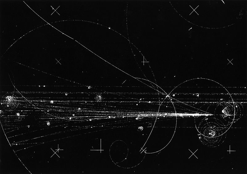
Image Hydrogen bubble chamber Fermilab: Proton with 300 GeV energy producing 26 charged particles in the 30 inch hydrogen bubble chamber at Fermilab. Source: Wikimedia Commons
[1] Einstein, A. (1905) ‘Zur Elektrodynamik bewegter Körper’, Annalen der Physik, 322(10), pp. 891–921. doi: 10.1002/andp.19053221004.
This is a repost. Slight errors in the parsing of LaTeX in the original article of 24 December 2018 have been corrected.
Well-known for their central role in Einstein’s Special Relativity, the Lorentz transformations are derived from the rotation of two frames of reference in standard configuration while time is taken to be an imaginary unit of spacetime. This is rarely seen in the wild. Not many undergraduate textbooks or online texts show the details of the working. Hence, this article.
One might think this means that imaginary numbers are just a mathematical game having nothing to do with the real world. (…) It turns out that a mathematical model involving imaginary time predicts not only effects we have already observed but also effects we have not been able to measure yet nevertheless believe in for other reasons. So what is real and what is imaginary? Is the distinction just in our minds?
S. Hawking[1]
Even though there are many derivations of the Lorentz transformations to be found in textbooks, in syllabi, and online, to me, one of the most elegant remains the version Henri Poincaré once alluded to[2], which Hermann Minkowski then toyed with a bit further—to put it unreasonably mildly—in what we now call Minkowski space, but is rarely expounded in the aforementioned places.
Henri Poincaré noted that, when the time axis of the two coordinate systems has been made imaginary, i.e. the imaginary axis in the complex plane, the transformations set forth by Hendrik Lorentz pop out automatically after a rotation of two reference frames in that complex plane.
In this document, we show how this is done. We assume the reader is familiar with complex numbers.
The aim is to derive the following set of Lorentz transformations:
where $(t,x,y,z)$ and $(t’,x’,y’,z’)$ are the coordinates of an event in two frames. The primed ($’$) frame is, seen from the unprimed frame, moving with speed $v$ in the $x$-direction. The speed of light in a vacuum is denoted by $c$. As a side note, the recurring term $(\sqrt{1-v^2/c^2})^{-1}$ is called the Lorentz factor and it is usually denoted by the letter $\gamma$.
Standard configuration
Figure 1: Two frames of reference in standard configuration. A two-dimensional depiction of Hermann Minkowski’s frame M and Albert Einstein’s frame E in standard configuration: the latter moves at speed v relative to the first in the direction of x. There is no motion in either the y- or z-direction. Note that some time has passed in this diagram. At time t=0, however, their origins were equal. In other words, at temporal coordinates t=t’=0, their spatial coordinates were the same, thus x=x’=0.
Suppose, Hermann is standing still on the ground. Albert is driving his car and moves away from Hermann at speed $v$. We then have two frames of reference. There is Hermann’s frame $\mathcal{M}$ (the ground), with its origin $O$ at Hermann’s feet on the ground. And there is Albert’s frame $\mathcal{E}$ (the car), with its origin at Albert’s bottom on his chair. Their frames of reference are said to be in standard configuration as depicted by Figure 1. This means that at time $t=0$ in frame $\mathcal{M}$ where $x=0$ as well, the time $t’=0$ and position $x’=0$ in frame $\mathcal{E}$, too, and that one frame is in uniform (constant) motion relative to the other. In other words, $\mathcal{M}$ and $\mathcal{E}$ are said to be synchronised when the spacetime coordinates
\[ (t,x) = (t’,x’) = (0,0). \]
Of course, in the real world, there are four spacetime coordinates for each frame, i.e. $(t,x,y,z)$ and $(t’,x’,y’,z’)$, but to make our calculations a little bit easier, we consider the temporal coordinate $t$ (and $t’$) and spatial coordinate $x$ (and $x’$) only.
So, looking at Figure 1, we can see from Hermann’s point of view – standing in the origin $O$ of $\mathcal{M}$ – that $\mathcal{E}$’s origin $O$ moves at speed $v$ relative to the $x$-axis of $\mathcal{M}$. Speed $v$, of course, just means that $\mathcal{E}$ moves at a certain amount of units of $x$ (say, metres) per a certain amount of units of $t$ (say, seconds). This is nothing new, but it is for our derivation of the Lorentz transformations important to repeat our secondary education for a little bit:
\[ v = \frac{\Delta x}{\Delta t}, \]
in Hermann’s frame of reference $\mathcal{M}$. More or less conversely, if we want to calculate how many spatial units frame $\mathcal{E}$’s origin has moved from frame $\mathcal{M}$’s origin, we rewrite the last equation into the perhaps more familiar law of uniform motion:
\begin{equation} \Delta x = v \Delta t, \label{eq:x=vt} \end{equation}
in Hermann’s frame of reference $\mathcal{M}$.
As a side note, do realise that to Albert, his car is not moving at all; he is sitting in it. (Rather, it is the rest of the world that is moving with respect to his car and himself.) If the car were moving with respect to Albert, an accident with potentially serious consequences would be impending. So, for Albert’s sake, his speed within his own frame $\mathcal{E}$ (the car) is expressed as $v’=0$, as long as he stays put and buckled up in his chair. And so, the law of uniform motion of Albert, within his frame $\mathcal{E}$, becomes:
\[ \Delta x’ = v’ \Delta t’ = 0 \Delta t’=0. \]
Invariances
If $\mathcal{E}$ is in constant motion with respect to $\mathcal{M}$, in one direction, the $x$-direction, as expressed in Equation \eqref{eq:x=vt}, then, mathematically, we call this a geometric translation in the $x$-direction. In physics, it is called a translational motion in the $x$-direction.
Figure 2: Albert fires a photon. At time t=t’=0, Albert fires a photon P into direction x. Both the photon and Einstein’s frame E move into that same x-direction.
Suppose, at time $t=t’=0$, Albert activates his special on-board photoelectric cannon, firing exactly one photon $P$ in the $x$-direction. Figure 2 shows how the photon is travelling through the spaces of both frames of reference.
Looking at the diagram, we see that the spatial coordinates in the $y$-direction remain unchanged, $y=y’=0$, so we leave this out of our equations further on, to keep it simple. However, since $\mathcal{E}$ is moving with respect to $\mathcal{M}$ in the $x$-direction, we do know that $x\neq x’$ for $t>0$. And since we do not know for certain that $t=t’$ for $t>0$, only that $t=t’=0$, we will have to conclude that the position of $P$ differs:
Fortunately, accepting Einstein’s Voraussetzungen[3], we know that the speed of light, $c$, is the same for every frame of reference. Using Equation \eqref{eq:x=vt}, $x=vt$, and the fact that $v=c$, in this case, we can write for the distance travelled of photon $P$ – the yellow line in the diagram – in the coordinates of the respective frames of reference: \begin{align} \text{in Albert’s }\mathcal{E}\text{: }\Delta x’ &= c\Delta t’, \\ \text{in Hermann’s }\mathcal{M}\text{: }\Delta x &= c\Delta t. \end{align}
As it is possible for any coordinate system to have points which lie on the negative side of the origin of a spatial dimension such as $x$ in our case, and thus for light to travel in the negative $x$-direction, we simply square both equations to always obtain a positive value.
This is a beautiful result, because it tells us that no matter what frame of reference you happen to be in, besides $c$, Albert and Hermann agree on the quantity $(\Delta x)^2 – (c\Delta t)^2$, despite the fact that the coordinates of $P$ are not necessarily the same in every frame of reference as we saw in \eqref{eq:coordinates of P}. In other words, both $c$ and $(\Delta x)^2 – (c\Delta t)^2$ are said to be invariant.
You might wonder, what is this invariant quantity $(\Delta x)^2 – (c\Delta t)^2$, exactly? Well, this will be discussed in another post called What is a spacetime interval? And now, we might have just told you what it is. Anyway, let us move on to deriving the Lorentz transformations, and just keep in mind that $(\Delta x)^2 – (c\Delta t)^2$ is a wonderfully invariant quantity, equal in both frames of reference. Let us move on to imaginary time.
Wick rotation and imaginary time
Number sets
Figure 3: real number line. A segment of the real number line, the set R of all real numbers, which goes on to infinity on either side.
As many of us should know, Figure 3 depicts (a segment of) the real number line, that is the set $\mathbb{R}$ of all real numbers. It formed the culmination of all the previous extensions of the then-known set of numbers. Starting with the natural numbers, a set usually denoted by $\mathbb{N}$, containing all positive integers, arisen from the natural act of counting, the numeric repertoire was then extended by the notion of negative integers. Instead of just 1,2,3, we could now also count to -1,-2,-3 etc. This extension is denoted by $\mathbb{Z}$. Needless to say that $\mathbb{N}\subset\mathbb{Z}$, but we just did anyway.
Of course, some people were clever, acknowledging the need for another extension: numbers which represented ratios, better known as rational numbers, such as 1/2, 1/-3, 1/4, -1/100, in other words, quotients of two integers. These numbers would sit in-between the integers in $\mathbb{Z}$. The symbol is $\mathbb{Q}$, and it is superfluous to add that $\mathbb{N}\subset\mathbb{Z}\subset\mathbb{Q}$.
While specified on a tablet, found in Susa (Iraq) in 1936, dated as used by Babylonians around 2000 BCE, that
it wasn’t until 1761 that a proof that $\pi$ is irrational was found by Johann Heinrich Lambert[3] meaning that it could not be constructed by any ratio of integers, as were many other numbers, such as $\sqrt{2}$. And so, yet again, an extension of the existing number line was needed. This was the aforementioned line representing the set $\mathbb{R}$, or, to be precise, $\mathbb{N}\subset\mathbb{Z}\subset\mathbb{Q}\subset\mathbb{R}$.
And then, in the 16th century, people such as rivals Tartaglia and Cardano independently recognised that solutions to cubic equations sometimes required the manipulation of square roots of negative numbers, such as $\sqrt{-1}$. Later, Bombelli developed proper operations such as addition and subtraction. A whole slew of subsequent mathematicians then developed over several decennia what is now known as the complex plane or gaussian plane[5], representing the set $\mathbb{C}$, extending the real number line with an imaginary axis with multiples of the imaginary unit $i=\sqrt{-1}$. (It is, obviously, the solution to the quadratic $x^2+1=0$.) We realise mentioning that $\mathbb{N}\subset\mathbb{Z}\subset\mathbb{Q}\subset\mathbb{R}\subset\mathbb{C}$ is utterly redundant at this point.
Translation and rotation
Figure 4: Number sets. Every consecutive number set is an extension of the previous one. We can move from a simpler set to a more complex one, for instance, by simply multiplying our current position by a number only present in the more complex set. Although it seems like we are tumbling from one set to another, we are really just ‘sliding left or right’, one-dimensionally, on the number line of the more complex set. This sliding is called a translation. Note: the amount of ticks in Q is much larger, but for obvious reasons of legibility, we only ticked every 1/2-ratio.
Let us have another look at the natural number line of $\mathbb{N}$. If we would want to convert the number 1 to a number that could not exist in $\mathbb{N}$ but could exist on the integer number line of $\mathbb{Z}$, let us then simply multiply the natural number 1 with a number from $\mathbb{Z}$, the negative integer $-1$. Since $1\times-1=-1$, we have transitioned from $\mathbb{N}$ to $\mathbb{Z}$. We ‘slid’ from 1 to $-1$, albeit in a different number set, which, mathematically, is the same as a translation by $-2$. This is easily expressed as starting from position 1, adding $-2$, and ending up at position $-1$ on the number line of, at least, $\mathbb{Z}$ (but not $\mathbb{N}$): $1+-2=-1$. Figure 4a aims to depict this.
We can do the same with moving from position $-1$ in $\mathbb{Z}$ to a number not in $\mathbb{N}$, nor in $\mathbb{Z}$, but at least in $\mathbb{Q}$ by simply multiplying by a fraction, such as $-1/2$, which is also a number not in $\mathbb{N}$, nor in $\mathbb{Z}$. This is, again, actually a translation, though now by adding $3/2$: $-1+3/2=1/2$. Figure 4b aims to depict this.
Similarly, transforming from position 1 in $\mathbb{Q}$ to $\mathbb{R}$, we multiply by, for instance, $\sqrt{2}$, which exists in $\mathbb{R}$ but not in $\mathbb{Q}$, and so, the result, $1\times\sqrt{2}=\sqrt{2}$ is in at least $\mathbb{R}$ but not in $\mathbb{Q}$, nor in $\mathbb{Z}$, nor in $\mathbb{N}$. The result is also a translation of $1+(\sqrt{2}-1)=\sqrt(2)$ in $\mathbb{R}$. Figure 4c aims to depict this.
Figure 5: Wick rotation of 1 and real time. Compared to the increasing complexity of the number lines in Figure 4, this one is the most complex so far. Two Wick rotations into the complex (number) plane C, where (a) the Re-axis is the real number line of the set R and the Im-axis is the imaginary unit line of the set C. Note that a complex number consists of both: a real part and an imaginary part. For instance, the complex number z is written in the form z = a + bi, with i = √-1. The real part of z is Re(z) = a, and the imaginary part Im(z) = b. And so, z = 1 + i, z = 1/2 + 3i, z = 3, are all complex numbers, where the latter has an imaginary part of Im(z) = 0, which we simply leave out as 0i = 0. A complex number is thus two-dimensional, embedded in a plane with a real axis and an imaginary axis. (b) Wick-rotating all real numbers on the time axis to the imaginary axis, transforms real time into imaginary time.
Note that, so far, the transformation of 1 or another number has involved a simple ‘sliding’ motion on the number lines, that is, one-dimensionally. Every time a new kind of number was introduced – the negative integers, ratios, and, lastly, the real numbers – a new set of numbers was created, and the number line evolved from discrete ($\mathbb{N}$) to a line continuum $\mathbb{R}$. The question is, what would be the next extension and what would it look like?
As stated earlier, in the 16th century it became clear that a new type of number was necessary to solve a slew of quadratic equations. Owing to people such as Wallis, Wessel, Argand, Buée, Mourey, Warren, Français, Bellavitis, Gauss, and Euler[5][6], the idea to extend the real number line of $\mathbb{R}$ with an imaginary, perpendicular number line came to fruition. This created the so-called complex (geometric) plane, sometimes called the $z$-plane, Gauss plane or Argand plane. It is important to note that transforming a real number in $\mathbb{R}$ to a complex number in $\mathbb{C}$ involves not a translation but a rotation. Multiplying a real number in $\mathbb{R}$, say 1, by a number that only exists in $\mathbb{C}$, say $i$, is the same as geometrically rotating our position 1 on the real axes by $\pi/2$ onto a position $i$ on the imaginary axis as is depicted in Figure 5a.
What if we did this with the entire real time axis in a space-time diagram as shown in Figure 5b? Every element of real time $t$ is multiplied by $i$. In other words, every part is rotated in the complex plane to become an entire imaginary axis of time $it$. This procedure is called a Wick rotation, named after theoretical physicist Gian Carlo Wick, who described such a procedure to solve problems in quantum and statistical mechanics[7].
This seems promising and is what Henri Poincaré alluded to fifty years earlier. Before we continue, we have to do one other little thing. It has something to do with units of measurement.
Minkowski diagrams
Figure 6: The distance-time-diagram we all grew up with. The independent variable time t as the x-axis, and the dependent variable distance, x, as the y-axis. Four particles are travelling through time and (one-dimensional) space, each with its own distance function of time, that is, each with its own speed. Note that P travels the most amount of distance over the same period, in other words, it is the fastest. Note that S travels exactly zero distance in that same amount of time.
We all grew up learning to read and use a type of diagram as depicted in Figure 6 during our physics classes. Time is put on the $x$-axis and distance $x$ is put on the $y$-axis. Somewhat confusingly, at first, as one might have gotten accustomed to using values of $x$ on the $x$-axis during the maths lessons. Of course, one learns that it is less about the names of variables and axes, rather, it is a matter of which is the independent and which is the dependent variable. The independent one, in this case, time $t$ (time flies, whether we want to or not), is then laid out over the axis called $x$ (which has not much to do with the variable named $x$), and the dependent one, a variable which happened to be named $x$, is projected onto the $y$-axis.
In this diagram, we see four particles. The fastest, $P$, is moving away in the $x$-direction (which is up, but not necessarily up into the sky, do realise that!) covering more units of $x$ than the other three after the same time $t_1$ has passed. This is why it has a steeper slope. The slowest one is the one that is not moving at all, the stationary particle $S$. It is moving in time, which is why it exists at time $t_1$, but, spatially, it does not exist at a certain amount of units of $x$ away from the origin. In fact, it exists in exactly the same place, the origin.
Figure 7: t–x-diagram. A physicist’s diagram, where distance in space, x, is projected on the x-axis and distance in time t is projected on the y-axis. Note that the faster a particle travels, the smaller the angle of its ‘line’ through space and time with the x-axis. If the particle is stationary, it only ‘travels’ through time and the angle with the x-axis is maximised at π/2. In other words, it just goes straight up.
Well, get yourself out of the habit: turns out that professional physicists like to flip the axes when it comes to time. In other words, they project the distance variable $x$ onto the $x$-axis, while the time variable $t$ almost invariably gets to be projected onto the $y$-axis. Yes, you heard it correctly. Time goes up in a physicist’s diagram. The esteemed professor Leonard Susskind, a theoretical physicist at Stanford University, even postulated, in part jokingly, during a lecture on the principle of least action that physicists are the only type of people who do this(beginfootnote)See, for instance, https://youtu.be/3apIZCpmdls?t=1447(endfootnote). And so, we flipped our diagram as you can see in Figure 7.
Speaking of units, usually, time is measured in seconds and distance in metres. Usually. Though, remember when you went to visit those new friends of your parents and that one of the first things they assured their hosts is that their hometown was actually not that distant and that it was just ‘a two-hour drive’? Distance, while usually measured in kilometres between two places, is now expressed in units of time. Assuming that people legally drive – from door to door – at an average speed of $100\text{ km/h}$, the distance will be around 200 km.
Why do people like to express distance in terms of units of time sometimes? Well, in some cases, people aren’t interested in the exact amount of kilometres, but rather tend to focus on how much of our valuable time a certain activity consumes, hence, an answer in units of time makes sense.
Astrophysicists do another interesting distance-as-time conversion when it comes to distances between galaxies, for instance. They work with visible light reaching their telescopes, and other types of radiation. Moreover, the distances they work with are ridiculously large, especially when expressed in kilometres. So, they work with light-years, which sounds like a unit of time, but denotes a certain distance. One light-year is the distance light travels in one Julian year, which is $365.25$ days. Light travels at a speed of $c=299792458\text{ ms}^{-1}$ in the vacuum. To calculate the number of seconds in a Julian year, we multiply the number of seconds in one minute times the number of minutes in one hour times the number of hours in one day times the number of days in one Julian year:
Using Equation \eqref{eq:x=vt} to calculate distance $x$ light travels in one Julian year, we get
\begin{align} x &= vt \text{, and because }v=c\text{, we write:} \\ x &= ct,\label{eq:x=ct} \\ &= 299792458\text{ ms}^{-1} \times 31557600\text{ s} \\ &= 9460730472580800\text{ m}, \\ &= 9460730472580.800\text{ km}. \end{align}
Since light travels this ridiculously large number of kilometres, it makes perfect sense for astrophysicists to use this fact to express the distance of stars and galaxies. This way, the nearest major galaxy, Andromeda, is only about $2.5$ light-years away. This is obviously more practical than $23651826181452\text{ km}$.
So, about describing distance in terms of units of time, we learnt that
in the case of a ‘normal scale’ distance such as between two towns, expressing a spatial distance in units of time makes it easier to compare with the amount of time one wishes to spend on travelling – it becomes like comparing time with time;
in the case of larger scale distances such as between two galaxies, expressing a spatial distance in light-units of time makes it easier to handle the impractically large numbers of the original units.
Let us go back at our diagram in Figure 7 again. The units of both axes are not the same. The $x$-axis is the distance, which is expressed in spatial units, such as metres. The $y$-axis is the time, expressed in temporal units, such as seconds. It is hard to compare the two: the units are not the same. Also, as particle physicists are usually dealing with extremely fast particles, near the speed of light, it is impractical to be using the standard units of time. So, physicists have devised a solution to both problems. Number one: what if we expressed time in units of distance? So, that is the other way around: not distance in units of time, but time in units of distance.
To do that, we simply use the formula as expressed in Equation \eqref{eq:x=ct}: $x=ct$. In other words, if we multiply time $t$ with the speed of light $c$, we get a distance. A little analysis of units checks out. If we multiply the units of the speed of light with the unit of time, we get a unit of distance:
Figure 8: ct. (a) The time axis is multiplied by c, so it is easier to compare time with space, i.e. time is expressed in units of distance. (b) We set c = 1 so that the so-called world line of any particle travelling at exactly the speed of light is always at an angle of π/4 with the x-axis. Or 45°, if you are into that sort of thing.
This does not mean we magically, qualitatively, or even hypothetically transformed the time dimension into a space dimension, even though this would be a perfect device for a cool work of science-fiction, but it does mean that we now express time in units of distance. And so, we label the $y$-axis with $ct$ as is shown in Figure 8.
Now, to tackle the second problem, where physicists work with particles whose motions approach the speed of light at distance scales smaller than an electron in the vicinity of black holes with forces greater than you would ever encounter, it is impractical to work with the ordinary distance and time units. Furthermore, they prefer to choose the units of $ct$ and $x$ such, that a ‘line’ of a photon, e.g. light, travelling through space and time, is always depicted at an angle of $\pi/4$ or $45^\circ$ with the $x$-axis. To do so, they set the speed of light to 1. So, $c=1$. What you get is a diagram as shown in Figure 8(b). Particle $P$ is a photon, thus travelling at the speed of light. So, its ‘line’ is at the exact angle of $\pi/4$ with both the $x$- and $y$-axis, i.e. the $x$ and $ct$, respectively. All the other particles thus travel at a certain ratio of $c$, i.e. a certain ratio of 1.
All this should tell you enough to figure out how fast a particle would be going if its ‘line’ would be drawn underneath that of $P$, i.e. at an angle smaller than $\pi/4$. And even though you should also be able to figure out if this is at all possible, we will tell you now that this is not possible.
By the way, the term ‘line’, which we use to describe the path a particle takes through space and time in our diagrams, is called a ‘world line’ as Hermann Minkowski would have wanted us to. And the diagrams of Figures ref7 and 8 are called Minkowski diagrams. They are also called spacetime diagrams, although there is a subtle difference: Minkowski diagrams are the subset of two-dimensional diagrams within the larger set of spacetime diagrams, which contains the 3D versions, and 4D, even.
Wick rotation revisited
Figure 9: from it to ict. (a) The Wick rotation of the real time axis ct to the imaginary time axis ict. We projected the coordinate system of Figure 8 onto ‘the floor’ to have the ct-axis then rotated to the imaginary ict-axis by multiplication by the imaginary unit i. (b) Consequently, the world line of P gets rotated onto the imaginary plane as well.
We are almost ready to derive the Lorentz transformations. The only thing we have to do, is Wick rotate the (real) time axis into the imaginary time axis, i.e. we rotate the $ct$-axis of Figure 8. So, we do as we did in the previous section Number sets: we multiply by the imaginary unit $i$ from the number set $\mathbb{C}$, thereby rotating the time axis of $\mathbb{R}$ into the complex plane $\mathbb{C}$ to become an imaginary axis of time.
Figure 9 offers a geometric representation of the whole operation. We projected our original coordinate system of Figure 8 onto ‘the floor’, so to speak. We left out particles $Q$, $R$, and $S$ to keep it legible. Wick-rotating the real time axis $ct$ by multiplying by the imaginary unit $i$ then yields the imaginary time axis $ict$. Automatically, the world line of $P$ rotates along into the complex plane. Note, that the spacetime coordinates of $P$ have changed a few times in this section. They were $(x_P,t_1)$, then they became $(x_P,ct_1)$, and have ended up to become $(x_P,ict_1)$. Just the way we like it.
Deriving the Lorentz transformations
Invariant world line in the complex plane
Figure 10: Wick-rotated M and E. Hermann’s M and Albert’s E frames of reference rotated at an angle θ relative to each other in the complex plane about their origin. We put a little square with sides marked I and II to aid us in our trigonometric calculations.
To end up with the Lorentz transformations as formulated in Equations \eqref{eq:Lorentz t-prime} and \eqref{eq:Lorentz x-prime} by rotating two frames of reference relative to each other in the complex plane – with an imaginary time axis – we refer to Figure 10.
In both frames, those of Hermann and Albert, a photon $P$ travels at speed $c$. By the second postulate of Einstein’s Special Relativity[3], we know that, somehow, the value for $c$, which is chosen to be 1 in our case, is the same in both frames of reference, even though one moves relative to the other, meaning the coordinates between the frames are unequal. In Figure 2, this is represented by $v$. In Figure 10, this is represented by an angle $\theta$.
We see that the coordinates of $P$ in $\mathcal{M}$ are $(\Delta x, ic\Delta t)$. In $\mathcal{E}$, they are $(\Delta x’, ic\Delta t’)$. They are related to each other by some proportion of angle $\theta$. Before we find that relation, we repeat our finding regarding Equation \eqref{eq:interval} in the section Invariances: the quantity $(\Delta x)^2 – (c\Delta t)^2$ is invariant. In our case, it is the interval $OP$ that is invariant, despite the fact that $P$ has different coordinates. In other words, geometrically, both $\mathcal{M}$ and $\mathcal{E}$ agree on the length of the yellow world line as you can see in Figure 10. We should proceed to show this.
Let us first write down the expressions for the invariant yellow world line $OP$ in both frames of reference:
\begin{equation} \Delta x^2 – c^2\Delta t^2 = (\Delta x’)^2 – c^2(\Delta t’)^2.\label{eq:interval in the complex plane} \end{equation}
This is the result we wanted. Whether it is with imaginary time or with real time, the quantity $\Delta x^2 – c^2\Delta t^2$ remains invariant. (Recall that $i^2=(sqrt{-1})^2=-1$.) Even in the complex plane, $\mathcal{M}$ and $\mathcal{E}$ agree on the magnitude of this quantity.
Coordinates in terms of the other coordinates
Let us now express the coordinates of $P$ in $\mathcal{E}$, i.e. $(\Delta x’,ic\Delta t’)$, in terms of angle $\theta$ and the coordinates of $P$ in $\mathcal{M}$, i.e. $(\Delta x,ic\Delta t)$. Firstly, we deduce an expression for $\Delta x’$ using Figure 10:
Lastly, as we want to find the relation between $\theta$ in the complex plane and $v$ in real spacetime, we forget $P$ for a moment and now write the expression for Albert himself, sitting in $O’$ of his frame $\mathcal{E}$ in terms of the coordinates of Hermann’s frame $\mathcal{M}$. In other words, how does Hermann see Albert move? Since Albert is not moving in his own frame $\mathcal{E}$, as we said earlier, after a certain amount of time $ic\Delta t$, his $\Delta x’=0$. So, by Equation \eqref{eq:delta x prime}, we write
To recapitulate, we have now obtained Equations \eqref{eq:delta x prime}, \eqref{eq:icdelta t prime}, which express the coordinates of $P$ in $\mathcal{E}$ in terms of angle $\theta$ and the coordinates of $\mathcal{M}$. Lastly, we obtained relation \eqref{eq:tan \theta} between angle $\theta$ and speed $v$ of Albert’s frame $\mathcal{E}$ as seen by Hermann in his frame $\mathcal{M}$. So, to restate, we obtained the following transformations:
Figure 11: Triangle tan θ. The geometric representation of Equation 9: an imaginary triangle with an imaginary slope tan θ, where Γ is the hypotenuse. Note that sin θ = (iv/c)/Γ and cos θ = 1/Γ.
The Lorentz transformations
Note that, algebraically, it is possible to write Equation \eqref{eq:tan \theta} as
which, geometrically, looks like 11. Note that $\sin\theta=(\mathrm{iv/c})/\Gamma$ and $\cos\theta=1/\Gamma$, so all we have to do now, is figure out what $\Gamma$ is. Using, again, the Pythagorean theorem:
Since in our configuration the differences are calculated from the origin, we can leave out the $\Delta$-sign, using just the coordinates, and so we obtain
And so, leaving out the $\Delta$-sign, using just the coordinates, we obtain \begin{equation} t’ = \frac{t-vx/c^2}{\sqrt{1-v^2/c^2}}, \end{equation}
which is, indeed, Equation \eqref{eq:Lorentz t-prime}.
It is important to note that, while not unusual to leave out the $\Delta$-sign, formally, it is incorrect: in Special Relativity there is no preferred (fixed) origin, hence, it is always about differences.
Lastly, we reiterate that the term $1/\sqrt{1-v^2/c^2}$ is often written as $\gamma$ and is called the Lorentz factor. Also, in some texts, the term $v/c$ is replaced by symbol $\beta$, yielding the following equivalent expressions of the Lorentz transformations:
\begin{align} ct’ &= \gamma(ct-\beta x), \\ x’ &= \gamma(x-\beta ct), \\ y’ &= y, \\ z’ &= z. \end{align}
Thanks to the imagination of many mathematicians and physicists before us, our ability to investigate, analyse, and calculate has become as supple and malleable as is, indeed, the fabric of the cosmos.
[1] Hawking, S. (2001) The universe in a nutshell. New York: Bantam Books. [2] Walter, S. (2014) Poincaré on clocks in motion. Amsterdam, Ne. [3] Einstein, A. (1905) “Zur Elektrodynamik Bewegter Körper,” Annalen der Physik, 322(10), pp. 891–921. doi: 10.1002/andp.19053221004. [4] Bailey, D. H. and Borwein, J. M. (2016) Pi : the next generation : a sourcebook on the recent history of pi and its computation. Switzerland: Springer. doi: 10.1007/978-3-319-32377-0. [5] Cooke, R. (2005) The history of mathematics : a brief course. 2nd edn. New York, N.Y.: Wiley. [6] Caparrini S. (2006) On the Common Origin of Some of the Works on the Geometrical Interpretation of Complex Numbers. In: Williams K. (eds) Two Cultures. Birkhäuser Basel, pp. 139-151. [7] Wick, G.C. (1954) Properties of Bethe-Salpeter Wave Functions. Physical Review, 96(4), pp. 1124-1134.
In these examples, the eigenvalues of matrices will turn out to be real values. In other words, the eigenvalues and eigenvectors are in $\mathbb{R}^n$.
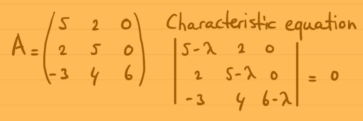
Suppose, we have the following matrix:
\begin{equation*}
\mathbf{A}=
\begin{pmatrix}
\phantom{-}5 & 2 & 0 \\
\phantom{-}2 & 5 & 0 \\
-3 & 4 & 6
\end{pmatrix}.
\end{equation*}
The objective is to find the eigenvalues and the corresponding eigenvectors.
1. Characteristic equation
Firstly, formulate the characteristic equation and solve it. The solutions are the eigenvalues of matrix $ \mathbf{A} $.
If $ \mathbf{I} $ is the identity matrix of $ \mathbf{A} $ and $ \lambda $ is the unknown eigenvalue (represent the unknown eigenvalues), then the characteristic equation is
\begin{equation*}
\det(\mathbf{A}-\lambda \mathbf{I})=0.
\end{equation*}
Written in matrix form, we get
\begin{equation} \label{eq:characteristic1}
\begin{vmatrix}
\phantom{-}5-\lambda & 2 & 0 \\
\phantom{-}2 & 5-\lambda & 0 \\
-3 & 4 & 6-\lambda
\end{vmatrix}
=0.
\end{equation}
Choose the row or column which are easiest to use to find the determinant of the matrix in equation \eqref{eq:characteristic1}. In other words, in this case, we will go down the last column as it contains the most zeros. This will decrease the length of the characteristic equation considerably:
\begin{align*}
&0\begin{vmatrix}\phantom{-}2 & 5-\lambda \\ -3 & 4 \end{vmatrix} \\
&\quad – 0\begin{vmatrix}5-\lambda & 2 \\ -3 & 4 \end{vmatrix} \\
&\qquad+ (6-\lambda)\begin{vmatrix}5-\lambda & 2 \\ 2 & 5-\lambda \end{vmatrix} = 0,
\end{align*}
and so
\begin{equation}
(6-\lambda)\begin{vmatrix}5-\lambda & 2 \\ 2 & 5-\lambda \end{vmatrix} = 0.
\end{equation}
Simplifying further, gives
\begin{align*}
(6-\lambda)[(5-\lambda)(5-\lambda)-2^2] &= 0, \\
(6-\lambda)[25-5\lambda-5\lambda+\lambda^2-4] &= 0, \\
(6-\lambda)[\lambda^2-10\lambda+21] &= 0,
\end{align*}
enabling us to write a manageable form of the characteristic equation:
\begin{equation}
(6-\lambda)[(\lambda-3)(\lambda-7)] = 0,
\end{equation}
of which the solutions of $ \lambda $ are now apparent immediately:
\begin{equation}
\therefore \lambda = 6 \vee \lambda = 3 \vee \lambda = 7.
\end{equation}
Lastly, there are two ways to verify if the found values are correct. For instance, the sum of these values have to be equal to the trace of $\mathbf{A}$, which is the sum of the main diagonal of $\mathbf{A}$:
\begin{equation*}
\text{tr }\mathbf{A}=5+5+6=16.
\end{equation*}
And, indeed, the sum of the values of $\lambda$ is equal to 16 as well. We can also verify whether the product of the values of $\lambda$ is equal to $\det\mathbf{A}$:
\begin{align*}
\det\mathbf{A} &= 0\begin{vmatrix}\phantom{-}2&5\\-3&4\end{vmatrix} \\
&\qquad -0\begin{vmatrix}\phantom{-}5&2\\-3&4\end{vmatrix} \\
&\qquad\quad +6\begin{vmatrix}5&2\\2&5\end{vmatrix} \\
&= 6\begin{vmatrix}5&2\\2&5\end{vmatrix} \\
&= 6(5^2-2^2) \\
&= 126.
\end{align*}
And, indeed, the product of the values of $\lambda$ is equal to $6\cdot3\cdot7=126$.
2. Specify the eigenvalues
The eigenvalues of matrix $ \mathbf{A} $ are thus $ \lambda = 6 $, $ \lambda = 3 $, and $ \lambda = 7$.
3. Eigenvector equations
We rewrite the characteristic equation in matrix form to a system of three linear equations. As it is intended to find one or more eigenvectors $ \mathbf{v} $, let
\begin{equation} \label{eq:v01}
\mathbf{v} =
\begin{pmatrix}
x_1 \\
x_2 \\
x_3
\end{pmatrix}
\end{equation}
and
\begin{equation}
(\mathbf{A}-\lambda\mathbf{I})\mathbf{v}=\mathbf{0}.
\end{equation}
In which case, we can write
\begin{equation} \label{eq:A-lambda I times v = 0}
\begin{pmatrix}
\phantom{-}5-\lambda & 2 & 0 \\
\phantom{-}2 & 5-\lambda & 0 \\
-3 & 4 & 6-\lambda
\end{pmatrix}
\begin{pmatrix}
x_1 \\
x_2 \\
x_3
\end{pmatrix}
=
\mathbf{0},
\end{equation}
which we can then write as a system of linear equations:
\begin{equation*}
\left\{
\begin{matrix}
(5-\lambda)x_1 + 2x_2 + 0x_3 &= 0, \\
2x_1 + (5-\lambda)x_2 + 0x_3 &= 0, \\
-3x_1 + 4x_2 + (6-\lambda)x_3 &= 0.
\end{matrix}
\right.
\end{equation*}
Simplifying this further, we have obtained the following eigenvector equations:
\begin{equation} \label{eq:eigenvectorvergelijkingen01}
\left\{
\begin{matrix}
(5-\lambda)x_1 + 2x_2 &= 0, \\
2x_1 + (5-\lambda)x_2 &= 0, \\
3x_1 – 4x_2 – (6-\lambda)x_3 &= 0.
\end{matrix}
\right.
\end{equation}
4. Substitute every obtained eigenvalue $\boldsymbol{\lambda}$ into the eigenvector equations4.1. Eigenvalue $ \boldsymbol{\lambda = 3} $
Let’s start with eigenvalue $ \lambda = 3 $. Substituting this into the eigenvector equations \eqref{eq:eigenvectorvergelijkingen01}, we get
\begin{align*}
(5-3)x_1 + 2x_2 &= 0, \\
2x_1 + (5-3)x_2 &= 0, \\
3x_1 – 4x_2 – (6-3)x_3 &= 0.
\end{align*}
We can simplify this to
\begin{align*}
2x_1 + 2x_2 &= 0, \\
2x_1 + 2x_2 &= 0, \\
3x_1 – 4x_2 – 3x_3 &= 0.
\end{align*}
The first equation and second equation reduce to $ x_1 = -x_2 $. Let’s substitute $ x_1 $ in the third equation.
\begin{align*}
3(-x_2) – 4x_2 – 3x_3 &= 0 \\
\therefore 7x_2 &= -3x_3.
\end{align*}
In other words, if $ x_2 = -3 $, then $ x_3 = 7 $, and $ x_1 = 3 $. And so, we can now fill in the values of $ \mathbf{v} $ in \eqref{eq:v01}:
\begin{equation}
\mathbf{v} =
\begin{pmatrix}
x_1 \\
x_2 \\
x_3
\end{pmatrix}
=
\begin{pmatrix}
\phantom{-}3 \\
-3 \\
\phantom{-}7
\end{pmatrix}.
\end{equation}
In other words, an eigenvector with eigenvalue $ \lambda = 3 $ is $ \begin{pmatrix}3 & -3 & 7\end{pmatrix}^T $. (Note: we deliberately write the words ‘an eigenvector’, as, for instance, the eigenvector $ \begin{pmatrix}54 & -54 & 126\end{pmatrix}^T $ is an eigenvector with this eigenvalue too. As long as $ x_1 = -x_2 $, and $ 7x_2 = -3x_3 $, in other words, as long as the ratios between $ x_1 $, $ x_2 $, and $ x_3 $ stay constant, it is an eigenvector of this eigenvalue. However, by convention we write the lowest possible integer values.)
We can check the validity of the eigenvector by calculating the inner product of $\mathbf{A}$ with the eigenvector. If all went well, the outcome will be equal to the inner product of the eigenvalue with the eigenvector, in other words, $ \mathbf{Av}=\lambda \mathbf{v} $. If we write this down in matrix notation (while, for clarity, simultaneously specifying which part is which variable), indeed, we get
\begin{align*}
& \underbrace{\begin{pmatrix}
\phantom{-}5 & 2 & 0 \\
\phantom{-}2 & 5 & 0 \\
-3 & 4 & 6
\end{pmatrix}}_{\mathbf{A}}
\underbrace{\begin{pmatrix}
\phantom{-}3 \\
-3 \\
\phantom{-}7
\end{pmatrix}}_{\mathbf{v}} \\
&=
\begin{pmatrix}
5\cdot3 + 2\cdot-3 + 0\cdot7 \\
2\cdot3 + 5\cdot-3 + 0\cdot7 \\
-3\cdot3 + 4\cdot-3 + 6\cdot7 \\
\end{pmatrix} \\
&=
\begin{pmatrix}
\phantom{-}9 \\
-9 \\
\phantom{-}21
\end{pmatrix}
=
\underbrace{3}_{\lambda}
\underbrace{
\begin{pmatrix}
\phantom{-}3 \\
-3 \\
\phantom{-}7
\end{pmatrix}}_{\mathbf{v}}.
\end{align*}
4.2. Eigenvalue $ \boldsymbol{\lambda = 6} $
In the same vein, we replace $ \lambda = 6 $ in the eigenvector equations of \eqref{eq:eigenvectorvergelijkingen01}. We then write the following three linear equations:
\begin{align*}
(5-6)x_1 + 2x_2 &= 0, \\
2x_1 + (5-6)x_2 &= 0, \\
3x_1 – 4x_2 – (6-6)x_3 &= 0.
\end{align*}
We can simplify further:
\begin{align*}
x_1 &= 2x_2, \\
2x_1 &= x_2, \\
3x_1 &= 4x_2.
\end{align*}
We see that $ x_1 = x_2 = 0 $ is the only solution to this system of simultaneous equations. As $ x_3 $ always multiplies by 0 (which is why it does not appear anymore in this system), $ x_3 $ can take any value. An eigenvector to eigenvalue $ \lambda = 6 $ is therefore simply $ \begin{pmatrix}0 & 0 & 1\end{pmatrix}^T $. Checking this using the inner product of matrix $\mathbf{A}$ with $ \begin{pmatrix}0 & 0 & 1\end{pmatrix}^T $, we get, indeed, $\lambda\mathbf{v}$:
\begin{align*}
&\begin{pmatrix}
\phantom{-}5 & 2 & 0 \\
\phantom{-}2 & 5 & 0 \\
-3 & 4 & 6
\end{pmatrix}
\begin{pmatrix}
0 \\
0 \\
1
\end{pmatrix} \\
&=
\begin{pmatrix}
\phantom{-}5\cdot0 + 2\cdot0 + 0\cdot1 \\
\phantom{-}2\cdot0 + 5\cdot0 + 0\cdot1 \\
-3\cdot0 + 4\cdot0 + 6\cdot1 \\
\end{pmatrix} \\
&=
\begin{pmatrix}
0 \\
0 \\
6
\end{pmatrix}
=
6
\begin{pmatrix}
0 \\
0 \\
1
\end{pmatrix}.
\end{align*}
4.3. Eigenvalue $ \boldsymbol{\lambda = 7} $
Substituting $\lambda=7$, yields
\begin{align*}
(5-7)x_1 + 2x_2 &= 0, \\
2x_1 + (5-7)x_2 &= 0, \\
3x_1 – 4x_2 – (6-7)x_3 &= 0.
\end{align*}
Working this further:
\begin{align*}
x_1 &= x_2, \\
x_1 &= x_2, \\
3x_1 – 4x_2 + x_3 &= 0.
\end{align*}
Substituting $ x_1 = x_2 $ into the third equation, we get
\begin{align*}
3x_2 – 4x_2 &= -x_3, \\
x_2 &= x_3.
\end{align*}
And so, we conclude
\begin{equation}
x_1 = x_2 = x_3.
\end{equation}
An eigenvector to the eigenvalue $\lambda=7$ is, thus, $\begin{pmatrix}1 & 1 & 1\end{pmatrix}^T$. Obviously, we can check this too:
\begin{align*}
&\begin{pmatrix}
\phantom{-}5 & 2 & 0 \\
\phantom{-}2 & 5 & 0 \\
-3 & 4 & 6
\end{pmatrix}
\begin{pmatrix}
1 \\
1 \\
1
\end{pmatrix} \\
&=
\begin{pmatrix}
\phantom{-}5\cdot1 + 2\cdot1 + 0\cdot1 \\
\phantom{-}2\cdot1 + 5\cdot1 + 0\cdot1 \\
-3\cdot1 + 4\cdot1 + 6\cdot1 \\
\end{pmatrix} \\
&=
\begin{pmatrix}
7 \\
7 \\
7
\end{pmatrix}
=
7
\begin{pmatrix}
1 \\
1 \\
1
\end{pmatrix},
\end{align*}
so, it is correct.
In these examples, the eigenvalues of matrices will turn out to be real values. In other words, the eigenvalues and eigenvectors are in $\mathbb{R}^n$.
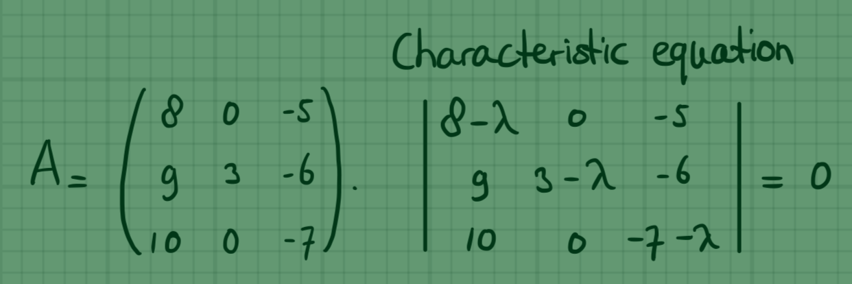
Suppose, we have the following matrix:
\begin{equation*}
\mathbf{A}=
\begin{pmatrix}
8 & 0 & -5 \\
9 & 3 & -6 \\
10 & 0 & -7
\end{pmatrix}.
\end{equation*}
The objective is to find the eigenvalues and the corresponding eigenvectors.
1. Characteristic equation
Firstly, formulate the characteristic equation and solve it. The solutions are the eigenvalues of matrix $ \mathbf{A} $.
If $ \mathbf{I} $ is the identity matrix of $ \mathbf{A} $ and $ \lambda $ is the unknown eigenvalue (represent the unknown eigenvalues), then the characteristic equation is
\begin{equation*}
\det(\mathbf{A}-\lambda \mathbf{I})=0.
\end{equation*}
Written in matrix form, we get
\begin{equation} \label{eq:characteristic1}
\begin{vmatrix}
8-\lambda & 0 & -5 \\
9 & 3-\lambda & -6 \\
10 & 0 & -7-\lambda
\end{vmatrix}
=0.
\end{equation}
Choose the row or column which are easiest to use to find the determinant of the matrix in equation \eqref{eq:characteristic1}. In other words, in this case, start with the first element of the second column, containing $ 3-\lambda $, as the rest of the elements in this row are zero. This will decrease the length of the characteristic equation considerably:
\begin{align*}
&-0\begin{vmatrix}9 & -6 \\ 10 & -7-\lambda \end{vmatrix} \\
&\quad + (3-\lambda)\begin{vmatrix}8-\lambda & -5 \\ 10 & -7-\lambda \end{vmatrix} \\
&\qquad- 0\begin{vmatrix}8-\lambda & -5 \\ 9 & -6 \end{vmatrix} = 0,
\end{align*}
and so
\begin{equation}
(3-\lambda)\begin{vmatrix}8-\lambda & -5 \\ 10 & -7-\lambda \end{vmatrix} = 0.
\end{equation}
Simplifying further, gives
\begin{align*}
(3-\lambda)[(8-\lambda)(-7-\lambda)-(-5)(10)] &= 0, \\
(3-\lambda)[-56-8\lambda+7\lambda+\lambda^2+50] &= 0, \\
(3-\lambda)[\lambda^2-\lambda-6] &= 0,
\end{align*}
enabling us to write a manageable form of the characteristic equation:
\begin{equation}
(3-\lambda)[(\lambda+2)(\lambda-3)] = 0,
\end{equation}
of which the solutions of $ \lambda $ are now apparent immediately:
\begin{equation}
\therefore \lambda = 3 \vee \lambda = -2 \vee \lambda = 3.
\end{equation}
Lastly, there are two ways to verify if the found values are correct. For instance, the sum of these values have to be equal to the trace of $\mathbf{A}$, which is the sum of the main diagonal of $\mathbf{A}$:
\begin{equation*}
\text{tr }\mathbf{A}=8+3-7=4.
\end{equation*}
And, indeed, the sum of the values of $\lambda$ is equal to 4 as well. We can also verify whether the product of the values of $\lambda$ is equal to $\det\mathbf{A}$:
\begin{align*}
\det\mathbf{A} &= -0\begin{vmatrix}9&-6\\10&-7\end{vmatrix} \\
&\qquad +3\begin{vmatrix}8&-5\\10&-7\end{vmatrix} \\
&\qquad\quad -0\begin{vmatrix}8&-5\\9&-6\end{vmatrix} \\
&= 3\begin{vmatrix}8&-5\\10&-7\end{vmatrix} \\
&= 31 \\
&= -18.
\end{align*}
And, indeed, the product of the values of $\lambda$ is equal to $3\cdot-2\cdot3=-18$.
2. Specify the eigenvalues
The eigenvalues of matrix $ \mathbf{A} $ are thus $ \lambda = -2 $ and $ \lambda = 3$.
3. Eigenvector equations
We rewrite the characteristic equation in matrix form to a system of three linear equations. As it is intended to find one or more eigenvectors $ \mathbf{v} $, let
\begin{equation} \label{eq:v01}
\mathbf{v} =
\begin{pmatrix}
x_1 \\
x_2 \\
x_3
\end{pmatrix}
\end{equation}
and
\begin{equation}
(\mathbf{A}-\lambda\mathbf{I})\mathbf{v}=\mathbf{0}.
\end{equation}
In which case, we can write
\begin{equation} \label{eq:A-lambda I times v = 0}
\begin{pmatrix}
8-\lambda & 0 & -5 \\
9 & 3-\lambda & -6 \\
10 & 0 & -7-\lambda
\end{pmatrix}
\begin{pmatrix}
x_1 \\
x_2 \\
x_3
\end{pmatrix}
=
\mathbf{0},
\end{equation}
which we can then write as a system of linear equations:
\begin{equation*}
\left\{
\begin{matrix}[r]
(8-\lambda)x_1 + 0x_2 – 5x_3 = 0, \\
9x_1 + (3-\lambda)x_2 – 6x_3 = 0, \\
10x_1 + 0x_2 + (-7-\lambda)x_3 = 0.
\end{matrix}
\right.
\end{equation*}
Simplifying this further, we have obtained the following eigenvector equations:
\begin{equation} \label{eq:eigenvectorvergelijkingen01}
\left\{
\begin{matrix}[r]
(8-\lambda)x_1 – 5x_3 &= 0, \\
9x_1 + (3-\lambda)x_2 – 6x_3 &= 0, \\
10x_1 + (-7-\lambda)x_3 &= 0.
\end{matrix}
\right.
\end{equation}
4. Substitute every obtained eigenvalue $\boldsymbol{\lambda}$ into the eigenvector equations4.1. Eigenvalue $ \boldsymbol{\lambda = -2} $
Let’s start with eigenvalue $ \lambda = -2 $. Substituting this into the eigenvector equations \eqref{eq:eigenvectorvergelijkingen01}, we get
\begin{align*}
(8-(-2))x_1 – 5x_3 &= 0, \\
9x_1 + (3-(-2))x_2 – 6x_3 &= 0, \\
10x_1 + (-7-(-2))x_3 &= 0.
\end{align*}
We can simplify this to
\begin{align*}
10x_1 &= 5x_3, \\
9x_1 + 5x_2 – 6x_3 &= 0, \\
10x_1 &= 5x_3.
\end{align*}
The first equation and third equation reduce to $ 2x_1 = x_3 $. Let’s substitute $ x_3 $ in the second equation.
\begin{align*}
9x_1 + 5x_2 -6(2x_1) &= 0 \\
\therefore 3x_1 &= 5x_2.
\end{align*}
In other words, if $ x_1 = 5 $, then $ x_2 = 3 $, and $ x_3 = 10 $. And so, we can now fill in the values of $ \mathbf{v} $ in \eqref{eq:v01}:
\begin{equation}
\mathbf{v} =
\begin{pmatrix}
x_1 \\
x_2 \\
x_3
\end{pmatrix}
=
\begin{pmatrix}
5 \\
3 \\
10
\end{pmatrix}.
\end{equation}
In other words, an eigenvector with eigenvalue $ \lambda = -2 $ is $ \begin{pmatrix}5 & 3 & 10\end{pmatrix}^T $. (Note: we deliberately write the words ‘an eigenvector’, as, for instance, the eigenvector $ \begin{pmatrix}30 & 18 & 60\end{pmatrix}^T $ is an eigenvector with this eigenvalue too. As long as $ 2x_1 = x_3 $, and $ 3x_1 = 5x_2 $, in other words, as long as the ratios between $ x_1 $, $ x_2 $, and $ x_3 $ stay constant, it is an eigenvector of this eigenvalue. However, by convention we write the lowest possible integer values.)
We can check the validity of the eigenvector by calculating the inner product of $\mathbf{A}$ with the eigenvector. If all went well, the outcome will be equal to the inner product of the eigenvalue with the eigenvector, in other words, $ \mathbf{Av}=\lambda \mathbf{v} $. If we write this down in matrix notation (while, for clarity, simultaneously specifying which part is which variable), indeed, we get
\begin{align*}
& \underbrace{\begin{pmatrix}
8 & 0 & -5 \\
9 & 3 & -6 \\
10 & 0 & -7
\end{pmatrix}}_{\mathbf{A}}
\underbrace{\begin{pmatrix}
5 \\
3 \\
10
\end{pmatrix}}_{\mathbf{v}} \\
&=
\begin{pmatrix}
8\cdot5 + 0\cdot3 + -5\cdot10 \\
9\cdot5 + 3\cdot3 + -6\cdot10 \\
10\cdot5 + 0\cdot3 + -7\cdot10 \\
\end{pmatrix} \\
&=
\begin{pmatrix}
-10 \\
-6 \\
-20
\end{pmatrix}
=
\underbrace{-2}_{\lambda}
\underbrace{
\begin{pmatrix}
5 \\
3 \\
10
\end{pmatrix}}_{\mathbf{v}}.
\end{align*}
4.2. Eigenvalue $ \boldsymbol{\lambda = 3} $
In the same vein, we replace $ \lambda = 3 $ in the eigenvector equations of \eqref{eq:eigenvectorvergelijkingen01}. We then write the following three linear equations:
\begin{align*}
(8-3)x_1 – 5x_3 &= 0, \\
9x_1 + (3-3)x_2 – 6x_3 &= 0, \\
10x_1 + (-7-3)x_3 &= 0.
\end{align*}
We can simplify further:
\begin{align*}
5x_1 &= 5x_3, \\
9x_1 &= 6x_3, \\
10x_1 &= 10x_3.
\end{align*}
We see that $ x_1=x_3=0 $ is the only solution to this system of simultaneous equations. As $ x_2 $ always multiplies by 0 (which is why it does not appear anymore in this system), $ x_2 $ can take any value. An eigenvector to eigenvalue $ \lambda = 3 $ is therefore simply $ \begin{pmatrix}0 & 1 & 0\end{pmatrix}^T $. Checking this using the inner product of matrix $\mathbf{A}$ with $ \begin{pmatrix}0 & 1 & 0\end{pmatrix}^T $, we get, indeed, $\lambda\mathbf{v}$:
\begin{align*}
&\begin{pmatrix}
8 & 0 & -5 \\
9 & 3 & -6 \\
10 & 0 & -7
\end{pmatrix}
\begin{pmatrix}
0 \\
1 \\
0
\end{pmatrix} \\
&=
\begin{pmatrix}
8\cdot0 + 0\cdot1 + -5\cdot0 \\
9\cdot0 + 3\cdot1 + -6\cdot0 \\
10\cdot0 + 0\cdot1 + -7\cdot0 \\
\end{pmatrix} \\
&=
\begin{pmatrix}
0 \\
3 \\
0
\end{pmatrix}
=
3
\begin{pmatrix}
0 \\
1 \\
0
\end{pmatrix},
\end{align*}
so, that is correct.
In these examples, the eigenvalues of matrices will turn out to be real values. In other words, the eigenvalues and eigenvectors are in $\mathbb{R}^n$.
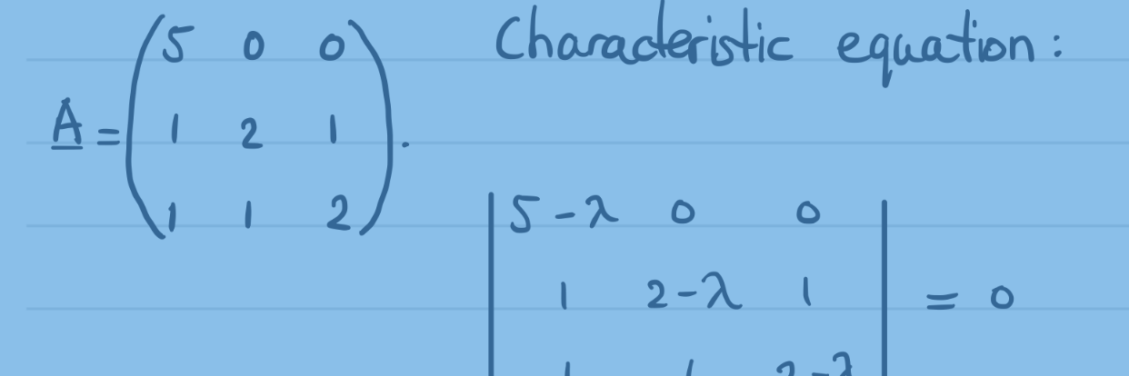
Suppose, we have the following matrix:
\[
\mathbf{A}=
\begin{pmatrix}
5 & 0 & 0 \\
1 & 2 & 1 \\
1 & 1 & 2
\end{pmatrix}.
\]
The objective is to find the eigenvalues and the corresponding eigenvectors.
1. Characteristic equation
Firstly, formulate the characteristic equation and solve it. The solutions are the eigenvalues of matrix $ \mathbf{A} $.
If $ \mathbf{I} $ is the identity matrix of $ \mathbf{A} $ and $ \lambda $ is the unknown eigenvalue (represent the unknown eigenvalues), then the characteristic equation is
\[
\det(\mathbf{A}-\lambda \mathbf{I})=0.
\]
Written in matrix form, we get
\begin{equation} \label{eq:characteristic1}
\begin{vmatrix}
5-\lambda & 0 & 0 \\
1 & 2-\lambda & 1 \\
1 & 1 & 2-\lambda
\end{vmatrix}
=0.
\end{equation}
Choose the row or column which are easiest to use to find the determinant of the matrix in equation \eqref{eq:characteristic1}. In other words, in this case, start with the first element of the first row, $ 5-\lambda $, as the rest of the elements in this row are zero. This will decrease the length of the characteristic equation considerably:
\begin{align*}
&(5-\lambda)\begin{vmatrix}2-\lambda & 1 \\ 1 & 2-\lambda \end{vmatrix} \\
&\quad – 0\begin{vmatrix}1 & 1 \\ 1 & 2-\lambda \end{vmatrix} \\
&\qquad+ 0\begin{vmatrix}1 & 2-\lambda \\ 1 & 1 \end{vmatrix} = 0,
\end{align*}
and so
\begin{equation}
(5-\lambda)\begin{vmatrix}2-\lambda & 1 \\ 1 & 2-\lambda \end{vmatrix} = 0.
\end{equation}
Simplifying further, gives
\begin{align*}
(5-\lambda)[(2-\lambda)(2-\lambda)-(1)(1)] &= 0, \\
(5-\lambda)[4-2\lambda-2\lambda+\lambda^2-1] &= 0, \\
(5-\lambda)[\lambda^2-4\lambda+3] &= 0,
\end{align*}
enabling us to write a manageable form of the characteristic equation:
\begin{equation}
(5-\lambda)[(\lambda-1)(\lambda-3)] = 0,
\end{equation}
of which the solutions of $ \lambda $ are now apparent immediately:
\begin{equation}
\therefore \lambda = 5 \vee \lambda = 1 \vee \lambda = 3.
\end{equation}
Lastly, there are two ways to verify if the found values are correct. For instance, the sum of these values have to be equal to the trace of $\mathbf{A}$, which is the sum of the main diagonal of $\mathbf{A}$:
\begin{equation*}
\text{tr }\mathbf{A}=5+2+2=9.
\end{equation*}
And, indeed, the sum of the values of $\lambda$ is equal to 9 as well. We can also verify whether the product of the values of $\lambda$ is equal to $\det\mathbf{A}$:
\begin{align*}
\det\mathbf{A} &= 5\begin{vmatrix}2&1\\1&2\end{vmatrix}-0\begin{vmatrix}1&1\\1&2\end{vmatrix}+0\begin{vmatrix}1&2\\1&1\end{vmatrix} \\
&= 5\begin{vmatrix}2&1\\1&2\end{vmatrix} \\
&= 5(2\cdot2-1\cdot1) \\
&= 15.
\end{align*}
And, indeed, the product of the values of $\lambda$ is equal to $5\cdot1\cdot3=15$.
2. Specify the eigenvalues
The eigenvalues of matrix $ \mathbf{A} $ are thus $ \lambda = 1 $, $ \lambda = 3 $, and $ \lambda = 5 $.
3. Eigenvector equations
We rewrite the characteristic equation in matrix form to a system of three linear equations. As it is intended to find one or more eigenvectors $ \mathbf{v} $, let
\begin{equation} \label{eq:v01}
\mathbf{v} =
\begin{pmatrix}
x_1 \\
x_2 \\
x_3
\end{pmatrix}
\end{equation}
and
\begin{equation}
(\mathbf{A}-\lambda\mathbf{I})\mathbf{v}=\mathbf{0}.
\end{equation}
In which case, we can write
\begin{equation} \label{eq:A-lambda I times v = 0}
\begin{pmatrix}
5-\lambda & 0 & 0 \\
1 & 2-\lambda & 1 \\
1 & 1 & 2-\lambda
\end{pmatrix}
\begin{pmatrix}
x_1 \\
x_2 \\
x_3
\end{pmatrix}
=
\mathbf{0},
\end{equation}
which we can then write as a system of linear equations:
\begin{equation*}
\left\{
\begin{aligned}
(5-\lambda)x_1 + 0x_2 + 0x_3 &= 0, \\
x_1 + (2-\lambda)x_2 + x_3 &= 0, \\
x_1 + x_2 + (2-\lambda)x_3 &= 0.
\end{aligned}
\right.
\end{equation*}
Simplifying this further, we have obtained the following eigenvector equations:
\begin{equation}
\left\{
\begin{aligned}
(5-\lambda)x_1 &= 0, \\
x_1 + (2-\lambda)x_2 + x_3 &= 0, \\
x_1 + x_2 + (2-\lambda)x_3 &= 0.
\end{aligned}
\right.
\label{eq:eigenvectorvergelijkingen01}
\end{equation}
4. Substitute every obtained eigenvalue $\boldsymbol{\lambda}$ into the eigenvector equations4.1. Eigenvalue $ \boldsymbol{\lambda = 1} $
Let’s start with eigenvalue $ \lambda = 1 $. Substituting this into the eigenvector equations \eqref{eq:eigenvectorvergelijkingen01}, we get
\begin{align*}
(5-1)x_1 &= 0, \\
x_1 + (2-1)x_2 + x_3 &= 0, \\
x_1 + x_2 + (2-1)x_3 &= 0.
\end{align*}
We can simplify this to
\begin{align*}
4x_1 &= 0, \\
x_1 + x_2 + x_3 &= 0, \\
x_1 + x_2 + x_3 &= 0.
\end{align*}
The first equation reduces to $ x_1 = 0 $ as this is obviously its only solution. The other two equations are identical. As $ x_1 = 0 $, these reduce to $ x_2 = -x_3 $, in other words, if $ x_3 = 1 $, then $ x_2 = -1 $. And so, we can now fill in the values of $ \mathbf{v} $ in \eqref{eq:v01}:
\begin{equation}
\mathbf{v} =
\begin{pmatrix}
x_1 \\
x_2 \\
x_3
\end{pmatrix}
=
\begin{pmatrix}
\phantom{-}0 \\
-1 \\
\phantom{-}1
\end{pmatrix}.
\end{equation}
In other words, an eigenvector with eigenvalue $ \lambda = 1 $ is $ \begin{pmatrix}0 & -1 & 1\end{pmatrix}^T $. (Note: we deliberately write the words ‘an eigenvector’, as, for instance, the eigenvector $ \begin{pmatrix}0 & -13 & 13\end{pmatrix}^T $ is an eigenvector with this eigenvalue too. As long as $ x_2 = -x_3 $, in other words, as long as the ratio between $ x_2 $ and $ x_3 $ stays constant, it is an eigenvector of this eigenvalue. However, by convention we write the lowest possible values.)
We can check the validity of the eigenvector by calculating the inner product of $\mathbf{A}$ with the eigenvector. If all went well, the outcome will be equal to the inner product of the eigenvalue with the eigenvector, in other words, $ \mathbf{Av}=\lambda \mathbf{v} $. If we write this down in matrix notation (while, for clarity, simultaneously specifying which part is which variable), indeed, we get
\begin{align*}
& \underbrace{\begin{pmatrix}
5 & 0 & 0 \\
1 & 2 & 1 \\
1 & 1 & 2
\end{pmatrix}}_{\mathbf{A}}
\underbrace{\begin{pmatrix}
\phantom{-}0 \\
-1 \\
\phantom{-}1
\end{pmatrix}}_{\mathbf{v}} \\
&=
\begin{pmatrix}
5\cdot0 + 0\cdot-1 + 0\cdot1 \\
1\cdot0 + 2\cdot-1 + 1\cdot1 \\
1\cdot0 + 1\cdot-1 + 2\cdot1 \\
\end{pmatrix} \\
&=
\begin{pmatrix}
\phantom{-}0 \\
-1 \\
\phantom{-}1
\end{pmatrix}
=
\underbrace{1}_{\lambda}
\underbrace{
\begin{pmatrix}
\phantom{-}0 \\
-1 \\
\phantom{-}1
\end{pmatrix}}_{\mathbf{v}}.
\end{align*}
4.2. Eigenvalue $ \boldsymbol{\lambda = 3} $
In the same vein, we replace $ \lambda = 3 $ in the eigenvector equations of \eqref{eq:eigenvectorvergelijkingen01}. We then write the following three linear equations:
\begin{align*}
(5-3)x_1 &= 0, \\
x_1 + (2-3)x_2 + x_3 &= 0, \\
x_1 + x_2 + (2-3)x_3 &= 0.
\end{align*}
We can simplify further:
\begin{align*}
2x_1 &= 0, \\
x_1 – x_2 + x_3 &= 0, \\
x_1 + x_2 – x_3 &= 0.
\end{align*}
And here too, the first equation reduces to $ x_1 = 0 $. The second and third equation are thus both reducable to $ x_2 = x_3 $, meaning that if $x_3 = 1 $, then $ x_2 = 1 $. An eigenvector to the eigenvalue $ \lambda = 3 $, is therefore simply $ \begin{pmatrix}0 & 1 & 1\end{pmatrix}^T $.
If we check this by calculating the inner product of matrix $\mathbf{A}$ with $ \begin{pmatrix}0 & 1 & 1\end{pmatrix}^T $, indeed, we obtain $\lambda\mathbf{v}$:
\begin{align*}
&\begin{pmatrix}
5 & 0 & 0 \\
1 & 2 & 1 \\
1 & 1 & 2
\end{pmatrix}
\begin{pmatrix}
0 \\
1 \\
1
\end{pmatrix} \\
&=
\begin{pmatrix}
5\cdot0 + 0\cdot-1 + 0\cdot1 \\
1\cdot0 + 2\cdot-1 + 1\cdot1 \\
1\cdot0 + 1\cdot-1 + 2\cdot1 \\
\end{pmatrix} \\
&=
\begin{pmatrix}
0 \\
3 \\
3
\end{pmatrix}
=
3
\begin{pmatrix}
0 \\
1 \\
1
\end{pmatrix}.
\end{align*}
4.3. Eigenvalue $ \boldsymbol{\lambda = 5} $
Substituting $\lambda=5$, yields
\begin{align*}
(5-5)x_1 &= 0, \\
x_1 + (2-5)x_2 + x_3 &= 0, \\
x_1 + x_2 + (2-5)x_3 &= 0.
\end{align*}
Working this further:
\begin{align*}
0x_1 &= 0, \\
x_1 – 3x_2 + x_3 &= 0, \\
x_1 + x_2 – 3x_3 &= 0.
\end{align*}
The first equation reduces to $0=0$, which is another way of saying that, logically, $x_1$ can take on any value as a solution to the equation. Working the other two equations some more too, we get
\begin{align*}
0 &= 0, \\
x_3 &= 3x_2 – x_1, \\
x_2 &= 3x_3 – x_1. \\
\end{align*}
These last two equations need some more work still. Substituting the second equation into the third, we get
\begin{align*}
x_2 &= 3(3x_2 – x_1)-x_1, \\
x_2 &= 9x_2 – 3x_1-x_1, \\
8x_2 &= 4x_1, \\
x_2 &= \frac{x_1}{2}.
\end{align*}
Substituting this result into the second equation, gives
\begin{align*}
x_3 &= 3\left(\frac{x_1}{2}\right)-x_1, \\
x_3 &= \frac{3x_1}{2}-x_1, \\
x_3 &= \frac{x_1}{2}.
\end{align*}
And so, we conclude
\begin{equation}
\frac{1}{2}x_1=x_2 = x_3.
\end{equation}
An eigenvector to the eigenvalue $\lambda=5$ is, thus, $\begin{pmatrix}2 & 1 & 1\end{pmatrix}^T$.
Obviously, we can check this too:
\begin{align*}
&\begin{pmatrix}
5 & 0 & 0 \\
1 & 2 & 1 \\
1 & 1 & 2
\end{pmatrix}
\begin{pmatrix}
2 \\
1 \\
1
\end{pmatrix} \\
&=
\begin{pmatrix}
5\cdot2 + 0\cdot1 + 0\cdot1 \\
1\cdot2 + 2\cdot1 + 1\cdot1 \\
1\cdot2 + 1\cdot1 + 2\cdot1 \\
\end{pmatrix} \\
&=
\begin{pmatrix}
10 \\
5 \\
5
\end{pmatrix}
=
5
\begin{pmatrix}
2 \\
1 \\
1
\end{pmatrix},
\end{align*}
so, it is correct.










.jpg)