Category: Mathematics

  • Spaces and dimensions

    Spaces and dimensions


    As is usually the case with scientific buzz words in everyday parlance, in books, in the cinema, on TV, and on the internet – like energy – the meaning of the word dimension rarely aligns with what mathematicians and physicists understand it to be. This day and age it’s rather uncommon to not have been exposed to phrases such as ‘higher’ or ‘other dimensions’. It’s likely you’ve used them yourself once or twice in your life. In this episode, we’ll explore what mathematicians and physicists mean when they talk about dimensions, and, more interestingly, the spaces they yield.

    Dimensions are not Universes

    In science-fiction or even everyday lingo, the word ‘dimension’ is often synonymous with entire worlds, or realms or (pocket) Universes. For instance, aliens may have come from another dimension. Or souls or ‘essences’ dwelling on a ‘higher plane of existence’ in another ‘dimension of reality’ are spoken about.

    On a regular basis, portals to other dimensions are opened from which exotic forms of matter and energy are extracted to benefit either the hero or the bad guy of the story.

    It’s also a favourite way to travel great distances within our reality. Just hop through a dimensional portal and out you come, back into our reality, only thousand kilometres away from where you started. Occasionally, you may also travel in time by flying through other dimensions.

    And, of course, other dimensions can be summoned into our own reality or, if the story goes that they have always been present inside our reality, they can be made visible by powerful minds. This is, again, alluding to dimensions being whole separate realms within our realm.

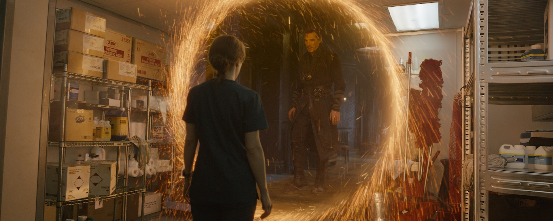
    Figure 1. Doctor Stephen Strange (Benedict Cumberbatch) is about to step into the Mirror Dimension as summoned within (or next to) our reality by his mentor, the Ancient One (Tilda Swinton), in the 2016 film Doctor Strange of the wildly popular Marvel Cinematic Universe (MCU).
    Figure 1. Doctor Stephen Strange (Benedict Cumberbatch) is about to step into the Mirror Dimension as summoned within (or next to) our reality by his mentor, the Ancient One (Tilda Swinton), in the 2016 film Doctor Strange of the wildly popular Marvel Cinematic Universe (MCU). License note. (Click to enlarge.)

    This whole section was just to let you know that what is meant by dimensions in most science-fiction stories is not what is meant in mathematics and physics. They are not realms, realities, worlds or pocket Universes. If we were to refer to realms, realities, worlds, and Universes, we would just say realms, realities, worlds, and Universes, but not dimensions.

    Ordinary spaces and dimensions

    So, what do mathematicians and physicists mean when they talk about dimensions?

    In many cases, they pertain to the actual directions you and I are able to travel in ordinary space. I prefer to think of birds and fish as gorgeous examples of being able to travel in all directions of space all by their own.

    They can fly from your left to your right and vice versa (first direction). They can fly head-on towards you and whizz by over your head and fly further behind you and vice versa (second direction). And, obviously, they can fly up from underneath you and they can keep on flying to way above your face. And vice versa (third direction).

    In many cases, all three directions are oriented perpendicularly with respect to each other. To use another word, they are orthogonal. All motion can be described as some combination of moving in these three orthogonal directions, i.e. orthogonal dimensions.

    In high school we have gotten all too familiar with these three dimensions. We were tortured with finding distances between vertices of a cube along the edges, the sides, and straight through the block. Of course, this is what modern gadgets and cinematography refer to when they use the term 3D, three-dimensional. In some way or form, all three orthogonal dimensions are either taken advantage of or simulated in a virtual way.

    Mathematically, the capability of travelling (or ‘transporting’) along these three orthogonal directions automatically give rise to a space, a topology, of some shape or form. Ordinary space is the space you and I are born in and have grown very much accustomed to.

    So, while dimensions may give rise to spaces, they are definitely not the same. Besides, while one dimension by itself technically yields a topology, a space, it’s still a one-dimensional space, meaning, no three-dimensional bodies are able to traverse this without being torn apart.

    Figure 2. In ordinary space, we have three dimensions in the x-direction, the y-direction, and the z-direction. In high school, we were to calculate the distance between points O and F, for instance.
    Figure 2. In ordinary space, we have three dimensions in the $x$-direction, the $y$-direction, and the $z$-direction. In high school, we were to calculate the distance between points $O$ and $F,$ for instance.

    Euclid and Descartes

    A very informal definition of dimensions is the number of coordinates needed to locate an object (in a space of some kind). So, on a flat surface (a plane), such as a ceiling, you need two coordinates to locate a fly. A fly can be 2 metres away from the left wall (the first direction) and 3 metres away from the back wall (the second direction, perpendicular to the first direction). Its coordinates are therefore (2,3). Hence, a plane is two-dimensional.

    In ordinary, three-dimensional space, we need three coordinates to locate a fly in a room. A fly can be 2 metres away from the left wall, 3 metres away from the back wall, and 1.5 metres up from the floor. Its coordinates are therefore (2,3,1.5).

    This was one of René Descartes’s great insights while lying in bed late in the afternoon or so the story goes. Hence, these numbers are called Cartesian coordinates. Descartes was pivotal to the development of what we now call the Cartesian coordinate system.

    The space to which these type of coordinates belong is called Euclidean space as the great Greek mathematician Euclid was the father of Euclidean or classical geometry.

    I think I can safely say that Euclid and Descartes enabled mathematics teachers to torment us with a whole slew of homework in order for us to fully explore the realm of Euclidean space in both two- and three-dimensional Cartesian coordinate systems.

    Figure 3. Home of Descartes in Utrecht, the Netherlands, where he wrote parts of his famous Discours de la Méthode. The house has been demolished. Nowadays, the place looks very different. (Click on the image for a link to the original Instagram post where you can also swipe for the photo of what is looks like today. Opens a new tab.)
    Figure 3. Home of Descartes in Utrecht, the Netherlands, where he wrote parts of his famous Discours de la Méthode. The house has been demolished. Nowadays, the place looks very different. (Click on the image for a link to the original Instagram post where you can also swipe for the photo of what is looks like today. Opens a new tab.)

    Space and time

    In real life, besides a position in ordinary space, you also need to specify when. Getting the coordinates to be inside an office located on the corner of two streets on the 24th floor (that’s the three dimensions of ordinary space right there) just isn’t enough. You also need a time-coordinate. When are you supposed to be there?

    One of my favourite books, Slaughterhouse-Five, or The Children's Crusade: A Duty-Dance with Death by Kurt Vonnegut mentions the Tralfamadorians who ‘were friendly’, and ‘could see in four dimensions’. They also ‘pitied Earthlings for being able to see only three.’ They were capable of observing all events at once.
    One of my favourite books, Slaughterhouse-Five, or The Children’s Crusade: A Duty-Dance with Death by Kurt Vonnegut mentions the Tralfamadorians who ‘were friendly’, and ‘could see in four dimensions’. They also ‘pitied Earthlings for being able to see only three.’ They were capable of observing all events at once.

    Einstein called the fact that you’re inside an office at a certain time an event. In other words, where, in ordinary, Cartesian coordinates, we talked about some thing being somewhere, Einstein had the insight to now only start talking about events taking place in terms of space and time, space-time – using space-time coordinates.

    When Einstein introduced the special theory of relativity, the German mathematician Hermann Minkowski realised this theory could also be understood geometrically in a four-dimensional space-time, where time is taken to be the fourth dimension. We now call this space Minkowski space. Note that we’re using the word ‘space’ in a broader sense: it doesn’t just encompass ordinary spatial dimensions but it now also includes a dimension of time (and, for technical reasons, isn’t Euclidean).

    By the way, another word mathematicians and physicists like to use is manifold. A manifold is a topological object which can take many shapes – such as a two-dimensional plane, a three-dimensional Euclidean space, four-dimensional Minkowski space or any other space you can mathematically think of.

    In Einstein’s general theory of relativity (gravity), we still work with four-dimensional space-time, except the shape of the space isn’t Minkowskian any more. The shape of the space is warped, curved, and stretched. In the best theory of gravity we have to date, we work on a so-called pseudo-Riemannian manifold, named after the great German mathematician Bernhard Riemann. The dimensions are still all the directions you can take on this manifold, i.e. the minimum amount of coordinates you need to locate an event. However, in this case, they are not necessarily oriented perpendicularly with respect to one another.

    Figure 4. In the film Interstellar (2014), director Christopher Nolan featured an object which had something to do with space and time.
    Figure 4. In the film Interstellar (2014), director Christopher Nolan featured an object which had something to do with space and time. (Click to enlarge.) If you haven’t seen the film and still intend to, do not read this footnote:(beginfootnote)Astronaut Joseph Cooper (Matthew McConaughey) finds himself in this spatial representation of space-time. All four dimensions of particular events in the past, present, and future of a room in his house, chopped up into manageable time chunks, are mapped onto an object (called a Tesseract) inside of a black hole (where the roles of space and time are reversed) through which Cooper can transport himself freely. This enables him to trickle information into the events of his choosing. In the still image above, you see many instances of the same room of his house with his daughter at different positions in time (which is the equivalent of different positions in space for Cooper).(endfootnote). License note.

    Four ordinary space dimensions

    Imagine a Pac-Man living on the surface of a sphere. To them, the world is flat. If they were to travel straight on – and on and on and on – eventually, they would be quite surprised to find themselves returning to the point where they started.

    Figure 5. Imagine being as flat as a Pac-Man, travelling on what seems to be a flat surface. You might be surprised to find you'd eventually end up where you started. If you had no knowledge of the three-dimensional concept of a sphere, that is. We do. We know that you'd return because that's what a sphere – or a circle, for that matter – does to your path. But what about our Universe? What if we would travel billions and billions of years in a straight line through the Universe? Would we end up where we started? Could our Universe be some kind of hypersphere? (Yes, technically, it's a glome, or an n-sphere, where n=3, and the space it's embedded in is n=1, not an hypersphere. Apologies to the mathematicians and physicists.)
    Figure 5. Imagine being as flat as a Pac-Man, travelling on what seems to be a flat surface. You might be surprised to find you’d eventually end up where you started. If you had no knowledge of the three-dimensional concept of a sphere, that is. We do. We know that you’d return because that’s what a sphere – or a circle, for that matter – does to your path. But what about our Universe? What if we would travel billions and billions of years in a straight line through the Universe? Would we end up where we started? Could our Universe be some kind of hypersphere(beginfootnote)Yes, technically, it’s a glome, or an n-sphere, where $n=3,$ and the space it’s embedded in is $n=1$, not a hypersphere. Apologies to the mathematicians and physicists.(endfootnote)?

    We, the three-dimensional beings most of us are, see them as a little surface, a shape, because we can see them ‘from above’, from the third dimension. We can also see how they’re travelling around the surface of a sphere. They don’t know what a sphere is. They only think of flat surfaces. To us, however, it’s quite logical they would eventually return to their point of origin.

    Okay, so, back to our 3D world. Imagine we travelled in a spaceship, always in a straight line through the Universe. Now imagine, after billions of years, we end up where we started: Earth. What happened? Could our Universe be some kind of sphere, only four-dimensional?

    The cover of the book The Fourth Dimension.
    I can recommend reading The Fourth Dimension: Toward a Geometry of Higher Reality. It became one of my favourite books in the 90s (though it came out in 1984). And there’s of course this book, to which many, such as Carl Sagan and Stephen Hawking, have referred in the past.

    While no experiment has proven the existence of a fourth spatial dimension (let alone five or six etc.), it is a wonderfully entertaining world for the mind to ponder about.

    Just to be absolutely sure: time is not the fourth dimension we’re talking about here. We were talking space – spatial dimensions. Quite often these two get confused: four-dimensional space-time is three spatial dimensions plus one time-dimension while four-dimensional space is four spatial dimensions without time.

    Abstract spaces

    There’s another way in which dimensions and spaces are used by mathematicians and physicists. Imagine an object having several properties at once: a position (in ordinary space), motion, direction of that motion, temperature, colour. To describe the state of this object, you need more than just four space-time coordinates. Suppose, its space-time coordinates are (0,1,1,1), in other words, it exists at time $t=0$ at position $(x=1; y=1; z=1)$.

    Did we describe the state of the whole object? No, we’re still missing some key properties here. It is in motion, so, it has a speed, say 10 m/s. That speed has a direction – this is why we say it has a velocity, which is speed and direction. Let’s say its velocity $v = -10 \text{ m/s},$ in other words, it has a speed of $10 \text{ m/s}$ to the left.

    Let’s say its temperature is 273.15 Kelvin, which is 0 ℃ and 32 ℉. And its colour is pure white. So, how many numbers do we need to describe the object’s state fully? Exactly, seven numbers (we count ‘white’ as a number).

    The coordinates (0,1,1,1,-10,273.15,white) are said to live in phase space, an abstract space where the properties of the object form the dimensions of that space. This particular phase space is seven-dimensional. Of course, that’s impossible to imagine, but mathematically, you can work very well with it.

    We gave an unusual example to emphasise that dimensions needn’t be related to spatial and temporal positions. However, usually, phase spaces are indeed used in the context of position and momentum.

    Figure 6. A sample trajectory through phase space is plotted near a so-called Lorenz attractor, a solution to the Lorenz system, which Edward Lorenz developed to model atmospheric convection. The colour of the solution fades from black to blue as time progresses, and the black dot shows a particle moving along the solution in time. The three-dimensional trajectory in phase space is shown from different angles to demonstrate its structure.
    Figure 6. A sample trajectory through phase space is plotted near a so-called Lorenz attractor, a solution to the Lorenz system, which Edward Lorenz developed to model atmospheric convection. The colour of the solution fades from black to blue as time progresses, and the black dot shows a particle moving along the solution in time. The three-dimensional trajectory in phase space is shown from different angles to demonstrate its structure.

    Another example of an abstract space is a so-called vector space where each coordinate does not just occupy a point in that space but that point also has a direction. An example of such a space is the velocity of wind. Each point in that space does not just have a value pertaining to the speed of the air and its location in ordinary space, it has a direction too.

    In the previous post, Complex numbers: an introduction, an entirely new kind of number line was introduced. All the spaces we just mentioned could very well contain complex dimensions. In fact, most of the time, they do. Especially in quantum mechanics. Complex numbers make up abstract complex vector spaces where wave functions thrive. Hilbert space is where it’s at, most of the time.

    The Standard model of quantum physics is based on groups of symmetrical transformations in complex space, called SU(3) $\times$ SU(2) $\times$ U(1). The S stands for special and denotes all possible transformations in complex space except for one particular kind. U(1) refers to a one-dimensional unitary circle group in the complex plane. The numbers indicate the number of dimensions in which these transformations take place. The number of dimensions of the entire system is much higher, though! The dimensionality of the abstract complex space which follows from a symmetry group such as SU(3) is $3^2-1=8.$ As you can see, compared to street corner vernacular, dimensions are very different in scientific context.

    In general, we can say that every manifold is a space. This needn’t pertain to spatial space. The minimum amount of dimensions needed to construct a path to a point on that manifold is the dimensionality of that space.

    There are so many more types of mathematical spaces, they’re too many to mention. Suffice to say, while they have nothing to do with our ordinary space – our real-world one, which we dwell in – all these abstract spaces are brilliant mathematical tools enabling us to do predictive calculations pertaining to phenomena taking place in our ordinary, real-world space.

    String theories

    An interesting beast among all of this is string theory. If you accept the premise that an elementary particle such as an electron is actually a spatially one-dimensional string vibrating in specific ways corresponding to the collection of properties of an electron, then more dimensions are automatically needed in order to describe all the particles in this way. Strings need a sufficient amount of freedom, degrees of freedom, to vibrate in unique ways to be able to encompass the entire zoo of elementary particles and their properties.

    Figure 7. The basic building blocks of the entire Universe, according to string theory. Unfortunately, while the theory is mathematically consistent, it cannot yet be (and hasn't been) proven to be correct in this Universe.
    Figure 7. The basic building blocks of the entire Universe, according to string theory. Unfortunately, while the theory is mathematically consistent, it cannot yet be (and hasn’t been) proven to be correct in this Universe.

    In various versions of the string theories, a varying number of dimensions are needed. These dimensions are spatial and invisible. Since we don’t experience these dimensions, it is hypothesised that they are extremely small and curled up. They’re not stretched out like our ordinary three spatial dimensions.

    Or they are so large that to us they don’t affect us in any way noticeable. Just as the curvature of Earth did not affect us when we were little as the Earth is so big compared to our movements.

    Unfortunately, the theory cannot be tested yet. For now it’s purely a mathematical exercise. Although many discoveries have been made in pure mathematics, no experiment has proven string theory to be true (string theory in all its variety, and I’m including superstring theories and M-theory here even though the hierarchy is the other way around). No extra dimensions have been found yet.

    There’s one honourable mention that I’d like to make. It’s the Calabi-Yau manifold, or the Calabi-Yau space. In superstring theory the manifold is hypothesised to encompass six invisible extra dimensions for the theory to work. The manifold is three-complex-dimensional or six-real-dimensional. I like it because it looks cool.

    None of this is proven; we seem to be stuck in this three-dimensional space with one direction of time. And, if you ask me, it’s likely that our three-dimensional space turns out to be a side product of something quantum.

    Figure 8. A Calabi-Yau manifold, named after Eugenio Calabi and Shing-Tung Yau. This is a complex space with complex dimensions. It yields applications in theoretical physics, most notably in superstring theory, where the manifold has six dimensions. Though not experimentally proven to be existing in our world, they do yield fascinating mathematical possibilities and puzzles.
    Figure 8. A Calabi-Yau manifold, named after Eugenio Calabi and Shing-Tung Yau. This is a complex space with complex dimensions. It yields applications in theoretical physics, most notably in superstring theory, where the manifold has six dimensions. Though not experimentally proven to be existing in our world, they do yield fascinating mathematical possibilities and puzzles.

    Spaces and dimensions

    There are so many different spaces with a variety of dimensions that you’d need a whole slew of posts to describe them all properly.

    What can we take away from all of this? Dimensions are not realms. In ordinary space, they are the directions in which objects can freely be transported. That’s three for our world.

    If you model time as a dimension, then we live in a four-dimensional space-time world. Except that you can’t freely move in time as there’s only one direction(beginfootnote)Time is definitely going to be a whole separate set of posts. Can’t wait.(endfootnote).

    Though many had hoped to find extra spatial dimensions, the largest experiment humankind has undertaken, the Large Hadron Collider at CERN, has not found a shred of evidence for them. Instead, it delivered convincing evidence that the current Standard Model of particle physics without extra dimensions is still correct.

    Nevertheless, to describe and predict phenomena in our Universe, it is almost always helpful to model their properties as extra dimensions. This has nothing to do with there actually being extra dimensions – this is probably where popular and esoteric culture get their inspiration from – but has everything to do with being able to do calculations in the abstract world of mathematics.

    In a previous post, for example, we assumed imaginary time as an extra dimension to mathematically derive a set of equations in the special theory of relativity. It doesn’t mean imaginary time is an actual extra dimension you can dip appendages or your consciousness into.

    In string theories, actual extra spatial dimensions are required for the theories to work. None of them can be tested as of yet (and none of them have been tested nor proven). It remains to be a beautiful, mathematical construct, but only mathematical.

    In future posts, we will be exploring geometry, pseudo-Riemannian manifolds, symmetry groups, and Hilbert space for loads more bits of maths and physics.

    Licenses

    The featured image in the title and Figures 1 are still images of Marvel Studio’s Doctor Strange (2014) and Figure 4 of Interstellar (2014), all copyrighted films. It is believed that screenshots may be exhibited under the fair use provision of United States copyright law.

    Figure 6. Lorenz attractor animation by Dan Quinn under CC BY-SA 3.0

    Figure 8. Calabi-Yau manifold by Lunch under CC BY-SA 2.5, created in Mathematica
  • Complex numbers: an introduction

    Complex numbers: an introduction


    Complex numbers have fascinated me since high school. Usually, it’s where we are taught about natural numbers, integers, rational, irrational, and real numbers but never about complex numbers. This post is for those who might be interested in an easy introduction into the realm, or rather, plane of complex numbers. And they’re not without practical significance either: no electronic device such as the one you’re using to read this post could have been built without physicists, electrical engineers, and computer scientists knowing anything about the gift of complex numbers from sixteenth century mathematicians.

    Blown away

    ‘There are such things as negative numbers’, explained my father to me when I must have been about six or seven years old since I was a second-year pupil in primary school. He explained the notion of negative possession when owing a certain number of marbles to someone which was greater than the number of marbles you physically carry with you. As this was one of those I-still-remember-where-I-was-when moments, like it was yesterday, I remember sitting on the floor besides the coffee table in the living room of our terraced house in the town of Emmeloord, which had been reclaimed just forty-three years earlier from the IJsselmeer, a lake formerly part of the North Sea.

    I clearly remember feeling exactly the same when he had told me earlier our planet wasn’t flat and when my Mum told me in the car yet a few months earlier, that we were living on the sea floor. The cap of my mind was blown away, yet again. It took a while before I managed to fold my slow and wet brain lobes around the notion that negative numbers existed, even though you couldn’t see them in the real world like you could ‘see’ regular numbers such as in lengths or the number of marbles(beginfootnote)Inexplicably, I had never considered the fact that temperature could get below 0 ℃, which it still did, back then in The Netherlands. We used to enjoy an outdoor activity called ice skating, on frozen lakes, ponds, rivers, and ditches.(endfootnote).

    I hastened to tell my primary school teacher excitedly about negative numbers. She just nodded and then told me to proceed with doing my homework on boring regular arithmetic. She had a point as I wasn’t very good at it.

    Fast forward to when I must have been about fifteen or sixteen when I read about complex numbers in a popular textbook about quantum mechanics. The fact that they were called ‘complex’ may have triggered my curiosity as I assumed that term pertained to it being very difficult, but mostly because, apparently, so-called imaginary numbers are a thing! I had that exact same feeling again. The cap of my mind had melted. The whole notion seemed to radiate some kind of magical power. What sorcery was this? Could this be a doorway to extra dimensions?

    The next day, I told my mathematics teacher, Mr Es – Es is not his actual name but it was his two-letter code in our high school timetable. I’ve always found it appropriate Es is also the symbol for the element Einsteinium in the periodic system. As his first name happened to be the same, my friends and I used to joke that we were on our way to the lessons of Albert Einstein.

    Mr Es did what every good teacher does when a student tells you something they get enthusiastic about: he encouraged it – in his case by lending me his old textbook from when he was a first-year mathematics student in Amsterdam. It was an introductory text about complex numbers at the level of undergraduate mathematics.

    The very textbook. (Click to enlarge.)

    I’m ashamed to say I kept it. It was one of those instances where, after the nth time of moving house, I realised, oh my god, I still have this!? It’s also true that I treasured it. It carries a special meaning to me. It signifies how, at least once in my lifetime, I felt acknowledged in what stirred me deeply at the time. A thing I couldn’t really share with friends or anyone close in general, I suddenly shared with someone very clever whose name was denoted by the symbol for Einsteinium.

    Thanks to the miracle of internet, we got back in touch, about twenty-five years later. I confessed I had always kept it and apologised. He had indeed wondered where it had been as he once wanted to show it to someone else. But I could keep it as he was cleaning out the attic anyway. And he was glad it had done something for me as he learnt about my current engagements in a bit of maths and physics.

    I felt guilty. I still do. Someone else could have enjoyed it just as much as I have. And now I have prevented that from happening through his book. So, whoever you are, my sincerest apologies.

    I hope, one day, I will be able to ignite sparks of joy for the beautiful mathematics of complex analysis to many others. I also hope you might experience at least a fraction of the amazement I felt and that the newly gained insight on the concept of ‘numbers’ might turn out to be beyond what you were able to imagine so far. So, let this be a beginning.

    Number sets

    A game of hopscotch drawn on the pavement with numbers on the tiles

    We all know and love (or hate, depending) the natural numbers: the whole numbers we count things with. 1, 2, 3, etc. Some mathematicians will want to include the number 0 while others don’t. In any case, this mathematical set of numbers is called the natural numbers and is denoted by the symbol $\mathbb{N}$.

    Then my father told me about the negative numbers, such as -1, -2, -3, etc. If you include the natural numbers and add to that these negative numbers, and add the number 0 to it (if you hadn’t already), then the result is an entirely new set of numbers called the integers, denoted by the symbol $\mathbb{Z}$.

    To denote that the set $\mathbb{N}$ is part of the larger set $\mathbb{Z}$, people use this symbol for subset, $\subset$. They will write $\mathbb{N}\subset\mathbb{Z}$, the natural numbers are a subset of the integers.

    Of course, there’s the ratio’s. The fractions. Between 1 and 2, there’s 1.5. So, in fraction-notation, that’s $\frac{3}{2}$. They’re obviously not whole numbers. They’re rational numbers because they can be represented by a ratio of integers. This number set is symbolised by $\mathbb{Q}$. We now have $$\mathbb{N}\subset\mathbb{Z}\subset\mathbb{Q}.$$

    It is interesting to note that, therefore, by this expression of subsets of subsets, even numbers such as 9 are rational numbers. On the surface, it’s not a fraction. Below the surface, however, it can be expressed as a ratio of integers: $9=\frac{9}{1}=\frac{18}{2}=\frac{36}{4}$, for example (and infinitely more).

    But wait, there’s more. Fractions such as 1.5 and 3.2 are finite. What if the decimals don’t end? What if you can’t write a particular kind of numbers as ratios, such as with the number $\pi$ or $\sqrt{2}$? These numbers are called the irrational numbers. They are all the numbers which aren’t rational. There’s no symbol for that(beginfootnote)Often, mathematicians circumvent the lack of a symbol by writing something like ​​​$\mathbb{R} \backslash \mathbb{Q}.$(endfootnote).

    Instead, there’s a symbol for all the natural numbers, the integers, the rational numbers, and the irrational numbers altogether(beginfootnote)Yes, indeed, my dear fellow mathematician, you thought correctly, I am skipping transcendental numbers here (and algebraic numbers, for that matter). As all transcendental numbers are irrational numbers but not all irrational numbers are transcendental, I decided it over-complicated things in what was supposed to be an introductory text on complex enough numbers anyway.(endfootnote). They’re called the real numbers and this set is denoted by $\mathbb{R}$. This is the set we’re all used to working with. We now have $$\mathbb{N}\subset\mathbb{Z}\subset\mathbb{Q}\subset\mathbb{R}.$$

    The set of real numbers $\mathbb{R}$ contains all the numbers. Or does it?

    A diagram of all the number sets in the shape of ellipses. The ellipse of R containing the ellipse of Q containing the ellipse of Z containing the ellipse of N.

    The secret of del Ferro, del Fiore, Tartaglia, and Cardano

    Well, you guessed it. Here they come, the complex numbers. Let’s do just a tiny bit of maths. Remember what the quadratic of a number was? And what a square root was? What is the square root of 64, in other words, $\sqrt{64}$? Yes, that’s 8. Because 8 times 8, or 8 squared, or $8^2$ equals 64.

    Okay, suppose $x^2 = 64$, what is $x$ then? Well, you do exactly the same thing, you un-square $x$ by taking its square root. And you have to do the same with the number after the equal sign. So, $\sqrt{x^2} = \sqrt{64}$, in other words, $x = 8$.

    Tartaglia

    Maybe you remember this comes in handy when calculating the lengths of the edges of your piece of land. Suppose, the surface area of your square piece of land is 64 square kilometre (or square miles). What is the length of an edge of that land? That’s 8 kilometre (or miles).

    All these calculations take place in the realm of $\mathbb{R}^+$, the positive part of all real numbers. Note that no surface area of a piece of land can be negative. In other words, a surface area of -64 square metres is nonsensical. Also, the square root of -64 has no solution. It’s not -8, because -8 times -8, or $(-8)^2$ is simply 64 again, because a negative number times a negative numbers equals a positive number as we proved in an earlier post.

    Cardano

    Sometime in the sixteenth century, somewhere in Italy, Scipione del Ferro, professor of the University of Bologna, solved a slightly different kind of equation. It was a so-called cubic equation. Where we basically found the solution to a quadratic equation such as $x^2 = 64$ from the top of our heads, he found solutions for a cubic equation such as $x^3 + x^2 + 6x + 3 = 0.$ Del Ferro was known for not wanting to publish any of his proofs and solutions. He kept a secret notebook and that was it.

    On his death bed, however, he told his pupil Antonio Maria del Fiore the secret to solving it. Del Fiore went on to challenge Niccolò Fontana Tartaglia, a mathematician residing in Venice at the time. Tartaglia had actually solved it himself before and trusted the formula to Gerolamo Cardano, the then Milan-based polymath and genius. Tartaglia messaged the solution in the form of a poem (no less!) but didn’t entrust the proof to him.

    Of course, Cardano was able to reconstruct the proof anyway. As he learnt that del Ferro had also found the solution, he then proceeded to publish it all in his Ars Magna from 1545, much to the chagrin of Tartaglia.

    So, what was the secret so many large minds had been secretive about? A new type of number.

    imaginary

    Let’s take a simpler example. Suppose, we have the following simplistic quadratic equation: $x^2 – 4 = 0$. To solve it, we ‘move’ the 4 to the other side of the equal sign, by adding 4 to both sides: $x^2 – 4 + 4 = 0 + 4$, which simply becomes $x^2 = 4$. If you apply the square root to both sides, you get $\sqrt{x^2} = \sqrt{4}$. The solution to this equation is thus $x=2$ or $x=-2$ (because $-2\times -2 = 4$ too).

    Good. Basically, the mathematicians of the sixteenth century opined that they should be able to solve a variation of this equation as well: $x^2 + 4 = 0$. Let’s bring the 4 again to the other side of the equal sign by subtracting 4 on both sides: $x^2 + 4 – 4 = 0 – 4$, which becomes $x^2 = -4$. Now, again, the question is, what is $x$?

    Let’s try and apply the square root to both sides again: $\sqrt{x^2} = \sqrt{-4}$. Halt. Stop. What is the square root of -4? What is the square root of a negative number?

    We have the same situation where we are to apply the square root of a negative surface area. The answer isn’t -2, because $-2\times -2 = 4$, not -4. What then?

    Before del Ferro, Tartaglia, and Cardano, people would have said that there simply is no solution. Thanks to them, however, we can solve it. The answer lies in the following definition: $$i^2=-1.$$

    This seemingly simple act enables us to solve $x^2=-4$. We can then write $x = 2i$ or $x = -2i$.

    Let’s take our first solution, $x = 2i$. If we square this, we get $x^2 = (2i)^2$, which we can also write as $x^2 = 2^2i^2$. Now, since $i^2 = -1$, we can substitute that to get $x^2 = 2^2(-1)$, which is, of course, $x^2 = -4$. Ecco!

    The same goes for the other solution, $x = -2i$. If we square this, we get $x^2 = (-2i)^2$, which we can write as $x^2 = (-2)^2i^2 = 4i^2 = 4(-1) = -4$. Ecco!

    So, you may ask, what devilish entity is this $i^2=-1$? The letter $i$ stands for ‘imaginary’ and so, $i$ is a so-called imaginary number.

    Now, because $i^2=-1$, you can also write(beginfootnote)Although, I actually prefer to use $i^2=-1$ over $i=\sqrt{-1}$ even though the latter has been mentioned in many school books. However, I believe it might lead to confusion. Since we have the rule that $\sqrt{a}\sqrt{b}=\sqrt{ab}$ where $a$ and $b$ are positive real numbers, you might try to apply this rule to negative real numbers, such as when $a=b=-1$. You would then get the incorrect statement $\sqrt{-1}\sqrt{-1} = \sqrt{(-1)(-1)} = \sqrt{1} = 1$, which is wrong as it should be equal to -1. That’s why I try to avoid using $i = \sqrt{-1}$ where I can.(endfootnote) that $i = \sqrt{-1}$. And that’s the crazy part: how can you calculate the square root of a negative number? How can you calculate the square root of a negative surface area? The answer is, you can’t. Not in the realm of the real numbers $\mathbb{R}$, that is. However, we’re not in Kansas anymore, Dorothy. We’re in a new land called the complex numbers. Bye $\mathbb{R}$, and welcome to $\mathbb{C}$.

    Here are some examples of complex numbers: $2i$, $\frac{2}{3}i$, $i\sqrt{2}$, $i \pi$, $-0.25i$. What’s more, you can add these imaginary numbers to a real number such as 3, like so: $3 + 2i$ or $3 + \frac{2}{3}i$ etc. These sums are their own answer. They are complex numbers.

    A complex number $z$ is of the form $z = a + bi$, where $a$ and $b$ are real numbers and $i^2 = -1$. The first real number, $a$, is called the real part of $z$. The last real number, $b$, is called the imaginary part of $z$. The set of all complex numbers is denoted by $\mathbb{C}$.

    And so, we now have

    $$\mathbb{N}\subset\mathbb{Z}\subset\mathbb{Q}\subset\mathbb{R}\subset\mathbb{C}.$$

    Note that every real number is a complex number but not every complex number is a real number. That is what one thing being a subset of another thing means. For instance, the real number 9 is a complex number where $b=0$. In other words, the real number 9 can be written as the complex number $9 + 0i$, which is simply 9, which thus happens to be a real number too.

    But $z = 3 + 2i$ is not a real number, because it has an imaginary part which is not equal to zero. So, $z$ is now exclusively a complex number.

    A diagram of all the number sets in the shape of ellipses. The ellipse of C containing the ellipse of R containing the ellipse of Q containing the ellipse of Z containing the ellipse of N.

    Complex plane

    Graphically, all the real numbers of $\mathbb{R}$ can be thought of as a point on the number line.

    A diagram depicting the real number line. Every point on this line represents a real number, such 0, 1, 2, 3 and the square root of 2, pi, and e.

    So, where do complex numbers reside?

    Owing to people such as Wallis, Wessel, Argand, Buée, Mourey, Warren, Français, Bellavitis, Gauss, and Euler[1], the idea to extend the real number line with an imaginary number line perpendicular to the real number line came to fruition. What you get is the so-called complex (geometric) plane, sometimes called the $z$-plane, Gauss plane or Argand plane.

    So, a complex number such as $z = 3 + 2i$, ‘contains’ the real number $3$ along the real axis, and the imaginary part, along the imaginary axis, sits at $2i$. A complex number is therefore always represented by a point in a two-dimensional space. Note that all the numbers from all the subset of complex numbers, i.e. $\mathbb{R}$ all the way down to $\mathbb{N}$, can also be represented by a point in this same two-dimensional complex space – it’s just that they all reside on the real axis.

    As you can -heh- imagine, doing calculations with complex numbers has become an exercise of geometry now! In fact, one of the most beautiful equations in mathematics (at least to my taste) pertains to trigonometry in the complex plane; it’s called Euler’s Formula.

    A diagram representing the complex plane. Perpendicular to the real number line is now a so-called imaginary axis with numbers such as i, 2i, 3i, pi-i, i square root of 2, etc. A complex number is now a point in on that surface.

    Not so imaginary

    It’s unfortunate that this number $i$ and any real number multiplication of it are called imaginary numbers. It was the renowned French philosopher and mathematician René Descartes who coined the term imaginary numbers because he considered them to be illusory. In fact, even Cardano had described them as ‘some recondite third kind of thing’[2].

    It’s unfortunate because ‘imaginary’ leads to semantic ambiguity. I get it: you would never see something like $\sqrt{-1}$ in the real world. But neither would you see $\sqrt{2}$ out in the wild, for that matter. And yet, it’s the exact length of the hypotenuse of a particular right triangle, which a skilled DIY person could make while you’re waiting. To me, ‘real’ numbers such as $\pi = 3.1415926535897 \dots$ without ever ending are as real as ‘imaginary’ numbers are (and vice versa). Circles are a real thing and $\pi$ can be used to do calculations on them. Well, with imaginary numbers you can do calculations on them just as well.

    Complex numbers are used in a variety of sciences. In Einstein’s relativity, which makes GPS navigation possible, you could make use of so-called imaginary time. This sounds like a concept straight from a science-fiction novel, however, imaginary time is a well-defined concept. In fact, in a previous post, we used this to derive the central set of equations in relativity, called the Lorentz transformations. See how the word ‘imaginary’ might invoke unwanted ambiguity?

    To make quantum mechanics work – the most successful theory to date – complex numbers are all over the place. Without them, the computer, mobile phone, tablet, TV, VCR, even your modern fridge – they wouldn’t have worked as no engineer would have been able to produce integrated circuits. The wave function is a complex function living in a complex separable Hilbert space, taking on complex probability amplitudes, evolving according to the Schrödinger equation, which itself is a complex equation.

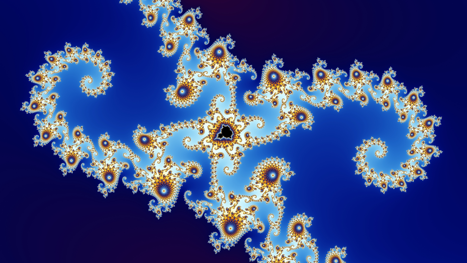
    In mathematics, one of the better-known areas of research where complex numbers play a central role is the study of complex dynamical systems. The featured image above is a detail of the famous Mandelbrot set. It’s a special collection of complex numbers, the projection of which you see plotted colourfully in the complex plane. The study of (complex) fractals also informs all kinds of patterns in nature and growth, even weather forecasts, and climate science – they’re all informed by complex-dynamical areas of mathematical interest. Also, we’ve used them in a previous post, calculating whether a lab centrifuge with $n$ available spots can be balanced out by a $k$ number of test tubes.

    A fun application of complex numbers is computer games. To calculate rotations in three-dimensional space, computer scientists make use of quaternions, which are an extension of the complex plane. A quaternion is an expression of the form $a + bi + cj + dk$, where $a,b,c,d$ are any old real numbers, and $i^2=j^2=k^2=-1$. However, this is perhaps an interesting subject for another bit of maths and physics.

    [1] Cooke, R. (2005) The history of mathematics : a brief course. 2nd edn. New York, N.Y.: Wiley.

    [2] Open University (2014) Essential mathematics 1. Milton Keynes: Open University.

    Images

    Featured image: Mandelbrot set – Step 6 of a zoom sequence by Wolfgang Beyer under CC BY-NC-SA 2.0; adapted to fit layout.

    Hopscotch Game by ncassullo.

    Niccolò Fontana Tartaglia. Rijksmuseum, Dutch National Museum. Public domain.

    Girolamo Cardano. Wellcome Images under CC BY 4.0.

  • Lab centrifuges and prime numbers

    Lab centrifuges and prime numbers


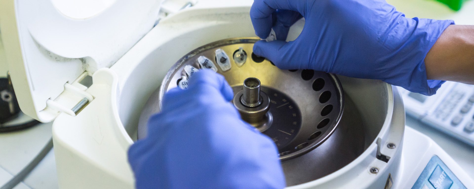
    When micro- or molecular biologists do research on viruses, bacteria, fungi, human or animal cells, one of the many instruments they will use is a laboratory centrifuge. This equipment allows them to separate substances contained within a test tube. This way scientists are able to obtain, for instance, purified enveloped viruses, such as the novel coronavirus, SARS-CoV-2. Or they can isolate nucleic acids, such as DNA.

    Often, the rotor of the machine rotates at incredible speeds. It is vital that the test tubes have been placed in a perfectly balanced way. If not, the machine might break down and potentially dangerous glass shards and substances might be flinging about(beginfootnote)Although sensors may be installed to prevent the machine from operating in case of force imbalance. See also the Final remarks down below.(endfootnote).

    Fortunately, there is a nifty way to calculate whether you can – in principle – place a certain number of test tubes in an evenly balanced way. To crack the code, we will use my favourite type of number: the prime numbers. Fun fact: this funky little trick wasn’t proven until fairly recently in 2010.


    NEW: Listen to the audio |


    The set-up

    Before we begin, we assume that the mass of each test tube, including their contents, is equal. Also, I would like to remark that, of course, we could do this the physics way, using angular velocity and torque and all that, but in this case, we’re going to be all mathy about it, or specifically, in a way, number-theoretical.

    Suppose, the machine can hold eight test tubes. Eight holes are positioned in a circle on the rotor bit of the machine.

    If we have just one test tube, there’s no way we can make it balanced. That much is clear. If we have two test tubes, however, no problem. They can be balanced easily. Just put one on either side precisely opposite each other. Three test tubes? Hm. I don’t see how. Whatever arrangement we try, it’s always going to be asymmetrical. What if you have four test tubes? Well, this is easy enough. Make it symmetric, like a square.

    Okay, so what about five test tubes? Well, that’s just the same as when we had the inverse of this, with three test tubes! That couldn’t be done, so, this can’t be done either.

    Six? Yeah, of course, we can do that. It’s just the same as having two test tubes, it’s just the inverse! Three on one side and three on the other side. Now you have two open spots on either side. Perfectly symmetrical, just like the inverse situation, where you had two test tubes and six open spots.

    Seven? No. You will have guessed it by now. Having seven test tubes is exactly the same as having just one test tube in a rotor with eight spots.

    And eight, well, of course, we can do eight. It’s also the exact same as having no test tubes at all. So, yes, that’s balanced.

    Do you see a pattern here? You might. Notice how the number of occupied spots and empty spots always complement each other.

    Prime factorization

    Just for clarity’s sake, I’m going to call whole numbers integers since that’s what they’re called in mathematics.

    So, I’m assuming we all know what a prime number is: an integer greater than 1 which cannot be formed by multiplying two smaller integers. In high school or even in primary school, you may have been taught that prime numbers are numbers which can only be divided by 1 or by itself (not including 1). So, prime numbers are 2, 3, 5, 7, 11, 13, 17 and so on.

    Prime factorization is writing down any non-prime integer as a multiplication of two or more prime numbers. The fundamental theorem of arithmetic states that any integer is either itself a prime number or can be written as a product of prime numbers. This is one of the reasons why they’re my favourite. Primes are the building blocks of any integer.

    So, for instance, we take the number 15. This number can be written as $ 15 = 3 \times 5 $. Or take 279. We can write $ 279 = 3 \times 3 \times 31 = 3^2 \times 31 $. Let’s take 16. This number can be written down as $ 16 = 2 \times 2 \times 2 \times 2= 2^4 $.

    As you can see, prime factorization is pulling apart a non-prime number into a product of prime numbers. We call the latter prime factors. 

    So, that’s what that is. One of the many applications of prime factorization is finding the greatest common divisor between two integers, for example. Or encrypting (and decrypting) secret files and messages. Here, we’re going to use it for calculating whether test tubes can be arranged in a balanced way.

    The trick

    Suppose, your machine has $n$ spots available. Suppose, $k$ is the number of test tubes. The number of empty spots is $n-k$. Here’s the trick.

    Determine the prime factors of $n$. If (and only if) $k$ can be written as a sum of these prime factors and the number of empty spots $n-k$ can be written as a sum of these prime factors, you can in principle balance the rotor.

    The mathematics

    It’s too technical to discuss at length the proof given by Gary Sivek in his 2010 paper (or here). However, the gist for the more mathematically inclined is available by clicking ‘expand’. You may skip this paragraph if this is (understandably) still too technical.

    Expand

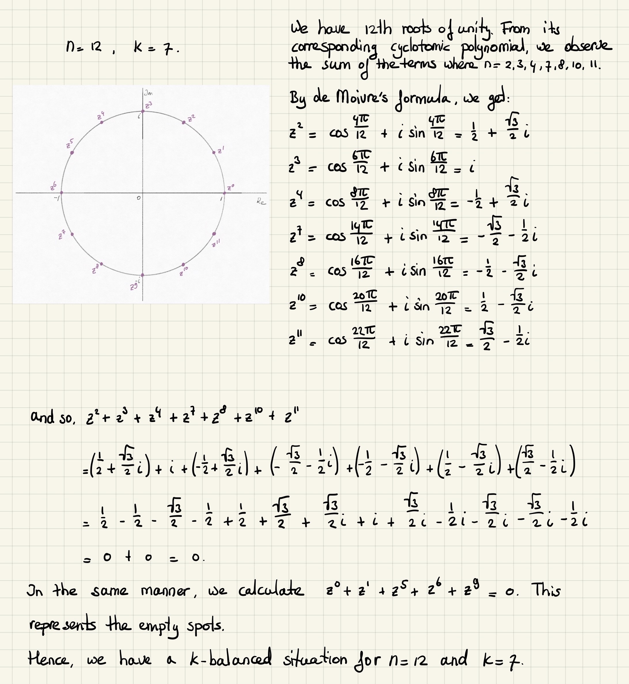
    Striving to obtain an $n$-th cyclotomic polynomial (or prime polynomial), we obtain a series of complex numbers $z^n$ which satisfy $z^n = 1$, all being $n$-th roots of unity where $n$ is the number of total spots on the centrifuge. We then map the test tubes onto the roots of unity in a non-overlapping way. As is well-known, the values of $z \in \mathbb{C}$ are given by $e^{\frac{2\pi i}{n} k}$, where $1 \leqslant k \leqslant n$.

    So, now we have $k$ roots of unity among the $n$-th roots of unity representing the occupied spots in the centrifuge.

    Sivek proved, using Leung’s and Lam’s Theorem, that if (and only if) the sum of the $n$-powered $k$ roots of unity and the sum of the $n$-powered $n-k$ roots ‘vanish’, i.e. are equal to zero (using good-old de Moivre’s formula, if you remember from your very first semester at uni), as long as $n \geqslant 2$ and $1 \leqslant k l\eqslant n-1 $, then balancing is a fact (where $k=0$ and $k=n$ were regarded to be trivial cases for obvious reasons).

    As you can see, no classical mechanics required.

    An example with eight roots of unity in the complex plane

    Obvious examples

    Suppose, we take our centrifuge which was capable of handling 8 test tubes. We have 6 test tubes. First thing we do is calculate which prime factors the number 8 has. We know this, it’s all 2s. So, the only prime factor of 8 is 2. We can write the number of test tubes, 6, as a sum of this prime factor 2: $6 = 2 + 2 + 2$. The number of empty spots, that’s $8-6 = 2$, is the prime factor itself! So, yes, if you have 6 test tubes, you can balance the machine.

    Let’s take 7 test tubes. Can this be written as a sum of the prime factors of 8? No, it can’t. Well, that’s it then. We cannot arrange the test tubes in such a way that it’ll be balanced out.

    A counter-intuitive example

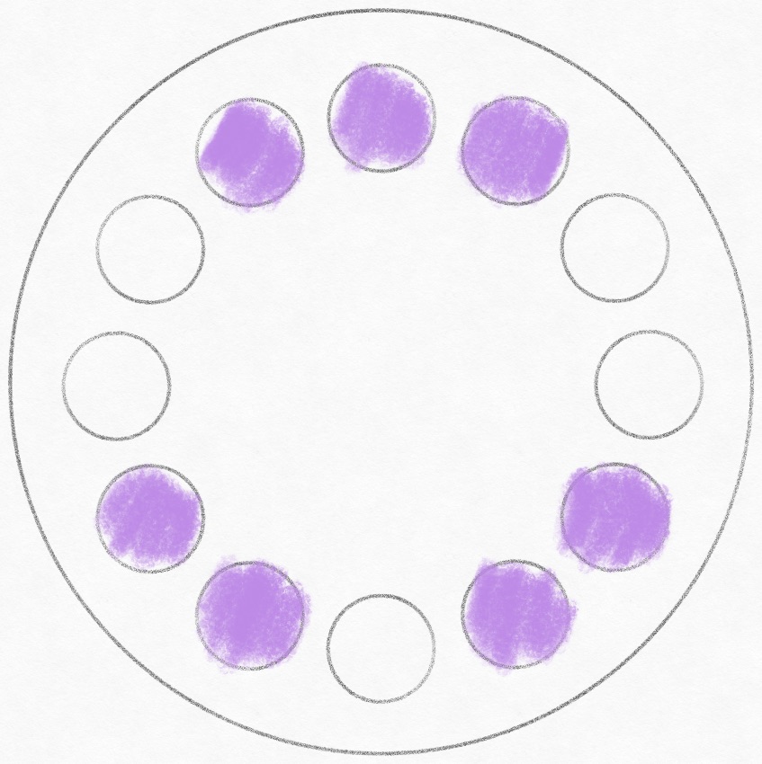
    Suppose, our centrifuge is capable of handling 12 test tubes in total. We only have 7 test tubes. Hm. Surely, we can imagine 6 test tubes working, but can we make a balanced arrangement with 7 test tubes?

    Let’s first do some prime factorization with 12. So, $ 12 = 2 times 2 times 3 = 2^2 times 3 $. In other words, the prime factors of 12 are 2 and 3.

    Now, can we write 7 as a sum of these prime factors? Yes, we can: $7 = 2 + 2 + 3$. Okay, so far, so good. Can we write the number of empty spots as a sum of these prime factors? Well, $12-7 = 5$. And yes, we can also write 5 as a sum of 2s and 3s: $5 = 2 + 3$.

    So, yes, we can balance 7 test tubes in a rotor with 12 spots! It’s likely this outcome wasn’t immediately apparent to you. If you were to see or draw a depiction and a working out of the arrangement yourself, however, I think it’ll become clear how this would work. Bonus points if you can draw a balanced configuration for 5 test tubes. Because you should know by now, you can.

    Bonus trick

    The beauty of it all is that all of the above does give us another quick way to assess whether we can balance the centrifuge. I’m going to be honest with you: it may be the easiest. If you can express the number of test tubes as the sum of two numbers of which you already know you can balance the rotor, then you can balance the rotor. Heh.

    Final remarks

    In real life, most machines have sensors to prevent force imbalances from taking over. The rotors have markings so that users won’t have to think about where to place the test tubes. Besides, in a university lab, you would simply make sure you prepare the number of samples which make a balancing act trivial. Moreover, many rotors contain three compartments containing sets of test tubes. This makes adjusting for mass variability much easier. And some machines, in hospital labs, for instance, have fully automated robots doing the heavy lifting.

    Therefore, the reason for why this type of mathematics is done, isn’t so much for the applicability as it is for the joy of exploring deep connections such as between prime numbers and complex geometry, if you will. It’s first and foremost a fun and fruitful exercise of human exploration of the lands of number theory, algebraic geometry, and finite fields, on the continent that is pure mathematics.

    Featured image by Michail Tzortzatos under CC BY-SA 4.0
    Spinning rotor by user musicalwoods under CC BY-SA 2.0

  • The Collatz Conjecture

    The Collatz Conjecture


    This Conjecture is probably one of the easiest to understand which hasn’t yet been proven in the history of mathematics. The beauty of this one is that a student in the last forms of primary school might very well be able to do the calculations while, thus far, not even the greatest mathematical minds have been able to prove if and why the Collatz Conjecture is true or not. The great, late Hungarian mathematician Paul Erdős has been quoted as saying: ‘Mathematics may not be ready for such problems.’[1]

    The rules

    There is some controversy over whether the prolific German mathematician Lothar Collatz was actually the first to come up with the idea in 1937, two years after his receiving his doctorate. It is also known as the ‘3n + 1 problem’, the Ulam conjecture, Kakutani’s Problem, the Thwaites Conjecture, Hasse’s Algorithm or the Syracuse Problem. If you were under the impression most of these refer to other, actual people then you are correct.

    As the rules of the Conjecture are so simple, it is likely many people have had the same idea independently of one another.

    Here are the rules:

    1. Take any positive, whole number – a positive integer, as it’s called.
    2. Do either of the following:
      • if the number is even, divide by 2;
      • if the number is odd, multiply by 3, add 1.
    3. Take the result and do either of the following:
      • if the result is 1, stop;
      • if the result is not 1, go back and do step 2 again but this time using the result to do either of the two operations, and so on.

    The Collatz Conjecture goes as follows: no matter which positive integer you start from, irrespective of the number of steps, you will always get 1 as final outcome.

    (Note that if you would continue to do the steps with 1, you would simply cycle back to 1 in just three steps until the end of times. I mean, that’s just boring and silly. So, stop at 1.)

    Example

    Let’s try it out. Let’s start with 10.
    10 is even; divided by 2 equals 5.
    5 is uneven; multiplied by 3 plus 1 equals 16.
    16 is even; divided by 2 equals 8.
    8 is even; divided by 2 equals 4.
    4 is even; divided by 2 equals 2.
    2 is even; divided by 2 equals 1. We’re there!

    This took us 6 steps. You can try a few numbers yourself if you’d like. Well, that is, have your computer, mobile phone or tablet do the boring work, which you can do here.

    Visualisation

    As you probably saw via the link above, we can also visualise the steps produced by the Collatz algorithm. We will quickly show a few alternatives before moving on to the most famous one, the Edmund Harriss visualisation (for which we wrote a JavaScript applet, yay!).

    Suppose, we would plot the progression of the results of our example. We started with 10. As you can see, the values fluctuate a bit before descending to 1:

    Have a look at the next one. We started at 8000. The numerical progression is then 8000 → 4000 → 2000 → 1000 → 500 → 250 → 125 → 376 → 188 → 94 → 47 → 142 → 71 → 214 → 107 → 322 → 161 → 484 → 242 → 121 → 364 → 182 → 91 → 274 → 137 → 412 → 206 → 103 → 310 → 155 → 466 → 233 → 700 → 350 → 175 → 526 → 263 → 790 → 395 → 1186 → 593 → 1780 → 890 → 445 → 1336 → 668 → 334 → 167 → 502 → 251 → 754 → 377 → 1132 → 566 → 283 → 850 → 425 → 1276 → 638 → 319 → 958 → 479 → 1438 → 719 → 2158 → 1079 → 3238 → 1619 → 4858 → 2429 → 7288 → 3644 → 1822 → 911 → 2734 → 1367 → 4102 → 2051 → 6154 → 3077 → 9232 → 4616 → 2308 → 1154 → 577 → 1732 → 866 → 433 → 1300 → 650 → 325 → 976 → 488 → 244 → 122 → 61 → 184 → 92 → 46 → 23 → 70 → 35 → 106 → 53 → 160 → 80 → 40 → 20 → 10 → 5 → 16 → 8 → 4 → 2 → 1.

    That’s a whole lot of numbers before the algorithm leads to 1. Hundred and fourteen steps, to be precise. This is what it looks like:

    As you can see, the whole plot fluctuates quite a bit. It’s a bit of a mess, really. There’s no distinct pattern other than it eventually converging to 1. As the values may become quite large very quickly, let’s plot the same graph in a semi-log grid. The y-axis is logarithmic, the x-axis remains linear.

    Just to humour ourselves, let’s reverse the step order, so that the plot is mirrored and converges to the value 1 in the bottom-left corner:

    As we’re not sure how many steps it might take before a sequence of numbers ends with 1, let’s also change the x-axis to a log scale. We get this:

    With this one, we can probably visualise a whole bunch of sequences! Lastly, let’s now plot a series of sequences! That is, firstly, we let our JavaScript applet calculate the sequence starting at 10000. Then we let it calculate the sequence starting at 9999. And so on, downwards, until it reaches 4. And then have it all plotted, all at once! To prevent it from becoming too dense, as several sequences will overlap each other, we add a little transparency to each plot. If the same ‘path’ has been taken, that path will appear ‘darker’. This is the result:

    This almost becomes some form of art. If you would frame this plot, without the titles, axes, and scales – just the plot – you could have a piece of geometrical art bearing the title ‘The Collatz Conjecture’ or something like that. I might do that, actually.

    With this applet you can generate your own ‘art’ like the one above.

    The Edmund Harriss visualisation

    Edmund Harriss, a mathematician working at the University of Arkansas, came up with a beautiful visualisation of progressions of Collatz sequences, which was featured on the mathematical YouTube channel Numberphile. We highly recommend following their channel.

    A screenshot of Numberphile’s video showing a partly hand-made version of Edmund Harriss’s visualisation

    The rules of visualisation are simple. While iterating through the Collatz rules, the algorithm goes as follows. If the current step is twice the value of the next step, rotate a fixed amount clockwise, otherwise rotate half of that fixed amount anticlockwise (and, again, stop at value 1). The result is a bundle of threads which looks like some sort of organic entity – messy and seemingly randomised within certain constraints, just like nature.

    We wrote a JavaScript applet to try and produce an approximation of his visualisation. We used it to produce the featured image at the top of this page. You can try it here yourself.

    Having visualised in several ways the kind of disorderly fashion in which the Collatz sequences progress, thus far, it may not seem surprising it has proven to be hard to crack the code. Well, the underlying mathematical code that is, not the JavaScript code.

    [1] Guy, Richard K. (2004). “E17: Permutation Sequences”. Unsolved problems in number theory (3rd ed.). Springer-Verlag. pp. 336–7. ISBN 0-387-20860-7. Zbl 1058.11001.

  • Proof that the square root of 2 is irrational

    Proof that the square root of 2 is irrational


    While it’s one of the most well-known and well-trodden proofs among proofs, the irrationality of $\sqrt{2}$ shouldn’t be lacking on a blog about mathematics and physics. So, here it goes.

    What is irrationality?

    For those who aren’t too familiar with mathematical jargon, let’s first discuss what it means to be irrational. Obviously, we’re not talking about the psychological attribute but the mathematical one.

    You might remember primary school when you had to learn about fractions such as

    \begin{equation} 1 = \frac{4}{12} + \frac{2}{3}. \end{equation}

    A practical application of a fraction is when you were reading a recipe for a delicious dish with a certain ratio of water and rice, which, even if you might not be aware of it all the time, can be written as a fraction, representing the ratio between water and rice. In fact, a fraction is a ratio.

    For instance, in order to cook the perfect, fluffy rice without the need to pour off excess water when the rice is cooked, the ratio is that for 1 cup of rice, you add 1.5 cups of water(beginfootnote)Rinse the rice thoroughly to remove the starch and dust for a nice fluffy texture. Add water by 1.5 times the used volume of rice. Add salt if you must. Bring the water to the boil as quickly as possible. Bring down the heat but keep the water bubbling softly. Give it one good stir. Put the lid on and don’t remove it for eight minutes. Don’t look inside; the water needs to stay in the pan. After eight minutes, shut off the heat and let it rest for another eight minutes. Still, don’t look. Keep the lid on the whole time. That’s it.(endfootnote) So, the fraction is $\frac{1}{1.5}$.

    Of course, it’s conventional to write a fraction using whole numbers (integers) only, so, $\frac{1}{1.5} = \frac{2}{3}$. Just multiply the numerator and the denominator by two. In other words, for 2 cups of rice, add 3 cups of water.

    If we use our calculator, we get $\frac{2}{3} = 0.666\dots$ There is no end to this number, but the number can be perfectly written down as a ratio: $\frac{2}{3}$.

    Of course, $\frac{2}{3}$ is the same as $\frac{4}{6}$, or $\frac{10}{15}$, or $\frac{200}{300}$, since, and this is crucial, all the other fractions (ratios) are simply multiples of our original fraction: they can all be simplified to their ‘simplest’ form, $\frac{2}{3}$. A slightly more technical way of saying this is that the fraction $\frac{2}{3}$ is the form in the lowest terms of the fraction $\frac{200}{300}$. It’s very important to remember this.

    Now we’ve arrived at what irrational numbers are.

    Premise 1. A number is irrational when it cannot be written as a ratio in lowest terms.

    Two of the more well-known examples of irrational numbers are $\pi$ and $\sqrt{2}$. If we use our calculator, we can see how there seems to be no numerical repetition in them. This is a quality that irrational numbers possess.

    Babylonian tablet clay tablet showing the root of 2 (credits below)

    Proof by contradiction

    So, how do we prove that $\sqrt{2}$ is irrational, i.e. it cannot be written as a ratio? We do this by contradiction: if the opposite of a statement is demonstrably false (and there are really only two options), then the statement itself must be true. In a previous article, we used the same strategy to prove that ‘minus minus is plus’.

    We will do that here, too.

    Even and odd

    Premise 2

    We will also use the fact that some number multiplied by 2 equals an even number. Take any number, odd or even, multiply that by 2, and you will get an even number. This isn’t rocket science, really, as a characteristic of an even number is that it’s divisible by 2. In our proof, we will use the symbol $k$ for ‘some number, any number, odd or even’ being multiplied by 2.

    Premise 3

    If you take the square of an odd number, the result is always odd. If you take the square of an even number, the result is always even. Conversely, if you take the root of an odd number, the result is always odd. The same idea goes for even numbers. Check in your head to see if that’s true (it is). We will provide a proof for that in another post.

    Okay, ready? Let’s go.

    Proof that the square root of 2 is irrational

    Anti-Premise 1. Suppose, by contradiction, that $\sqrt{2}$ can be written as some ratio in lowest terms: some (whole) number $a$ divided by some other (whole) number $b$ in lowest terms.

    In other words, suppose

    \begin{equation} \sqrt{2} = \frac{a}{b}. \end{equation}

    To make life a little bit easier, we get rid of the square root by squaring both sides of the equation:

    \begin{equation} 2 = \frac{a^2}{b^2}. \end{equation}

    If we rearrange this, we get

    \begin{equation} a^2 = 2b^2. \end{equation}

    Now, we see that $a^2$ is an even number as $b^2$ – whatever that number is – is multiplied by 2. It also means that $a$ cannot be an odd number – it’s even. Remember premise 3?

    Conclusion 1: $a$ cannot be odd – it’s even.

    We can then also state that $a = 2k$, where $k$ is some number, any number, odd or even. If we substitute that into equation (4), we get

    \begin{equation} (2k)^2 = 2b^2. \end{equation}

    If we rearrange that, we get

    \begin{equation} b^2 = \frac{(2k)^2}{2}. \end{equation}

    If we simplify this in one extra step, we get

    \begin{equation} b^2 = \frac{4k^2}{2} = 2k^2. \end{equation}

    This means that irrespective of what number $k^2$ is, because it’s multiplied by 2, the result is an even number. In other words, $b^2$ is an even number, which also means that $b$ is an even number.

    Conclusion 2. $b$ cannot be an odd number – it’s also an even number.

    Looking at conclusions 1 and 2, we arrive at

    Conclusion 3: $\frac{a}{b}$ is not a ratio in the lowest whole numbers as $a$ and $b$ can still be divided by 2.

    This is a contradiction. The fraction $\frac{a}{b}$ cannot both be the lowest fraction and not be the lowest fraction. Conclusion 3 contradicts Anti-Premise 1. Therefore, there is no fraction $\frac{a}{b}$ in lowest terms that exists that can be equal to $\sqrt{2}$. Hence, the original statement Premise 1 is true.


    Credentials of the Babylonian tablet clay tablet showing the root of 2: Photograph by Bill Casselman under CC BY-SA 3.0, and the Yale Babylonian Collection as the original holder of the tablet. A black and white rendition of Casselman’s own photograph of the Yale Babylonian Collection‘s Tablet YBC 7289 (c. 1800–1600 BCE), showing a Babylonian approximation to the square root of 2 (1 24 51 10 w: sexagesimal) in the context of Pythagoras’ Theorem for an isosceles triangle. The tablet also gives an example where one side of the square is 30, and the resulting diagonal is 42 25 35 or 42.4263888…(30 x square root of 2).


  • Finding the normal force in planar non-uniform circular motion using polar coordinates

    Finding the normal force in planar non-uniform circular motion using polar coordinates


    In this post, we will derive an expression for the normal force on a uniform mass which is in planar non-uniform circular motion using polar coordinates. Finding this expression is enormously useful to calculate under which circumstances a mass would be slung off its orbital path. Of course, there are numerous situations for which we should be able find the normal force. Here, we will look at a system as shown in Figure 1. Sometimes, obtaining an expression in terms of the variables given is not straightforward. You will find a useful trick in step 7 to arrive at an expression in terms of a simple $\theta$ instead of its secondary-order derivative $\ddot\theta$ which we initially obtain.

    This could be seen as an undergraduate-physics-level post. Download this article


    Notation

    We will apply Newton’s notation (the dot notation) whenever possible as this is the most compact form. For instance, if $\mathbf{x}$ is a vector, then its first-order and its second-order derivative with respect to time $t$ are denoted by

    \[ \dot{\mathbf{x}}\text{ and }\ddot{\mathbf{x}}, \]

    respectively. Where needed, in order to state explicitly that we are dealing with a time-derivative and to help in solving a time-integral for example, we will use Leibniz’s notation, i.e.

    \[ \frac{\text{d}\mathbf{x}}{\text{d}t}\text{ and }\frac{\text{d}^2\mathbf{x}}{\text{d}t^2}. \]

    Assignment

    Look at the system as sketched in Figure 1. Imagine we stand in front of this system. Mass $m$ is attached to a model string. At $t=0$, it rests at level with the centre of the cylinder with radius $R$ with the string draped over the top. A constant force $\mathbf{P}$ pulls the string downwards. At a later time $t$, mass $m$ has slid over the top with a coefficient of friction $\mu$. Let $\theta$ denote the angle between its initial and its current position, subtended at the centre of the cylinder. Calculate the normal force on $m$, and, hence, proof that the radius of the cylinder is irrelevant.

    Figure 1. The system

    Step 1. Force diagrams and unit vectors

    It is essential to draw force diagrams and unit vectors to define the acting forces and parameters. We choose the unit vectors to be the radial and the tangential vectors. This makes calculating most forces a lot easier. This is done in Figure 2.

    Figure 2. Force diagram and unit vectors at time $t>0$

    We identify the following forces on $m$:

    • $\mathbf{P}$ is the vector denoting the constant force pulling the model string,
    • $\mathbf{N}$ is the vector denoting the normal force acted on $m$ by the cylinder,
    • $\mathbf{F}$ is the vector denoting the frictional force,
    • $\mathbf{W}$ is the vector denoting the weight of $m$ as a result of the gravitational field of whatever planet the system is located,
    • $\mathbf{e}_r$ is the radial unit vector,
    • $\mathbf{e}_\theta$ is the tangential unit vector.

    Step 2. Apply Newton’s second law

    As this is a dynamical system, where $m$ is in non-uniform circular motion, we apply Newton’s second law, more specifically in the following form:

    \begin{equation}
    \sum\mathbf{F} = m\ddot{\mathbf{r}},
    \end{equation}

    where $\ddot{\mathbf{r}}$ is the rate of change of the rate of change over time, that is, the second time-derivative of the displacement vector $\mathbf{r}$ of mass $m$. We can now easily identify the constituents of the vector sum as we did that already in Step 1. And so, equation (1) becomes

    \begin{equation}
    m\ddot{\mathbf{r}} = \mathbf{P} + \mathbf{N} + \mathbf{F} + \mathbf{W}.
    \end{equation}

    Step 3. Rewrite the forces in terms of their magnitudes and unit vectors

    As pulling force $\mathbf{P}$ with magnitude $|\mathbf{P}|$ acts in the direction of tangential unit vector $\mathbf{e}_\theta$, we can write for $\mathbf{P}$:

    \begin{equation}
    \mathbf{P} = |\mathbf{P}|\mathbf{e}_\theta.
    \end{equation}

    Since we don’t have any other information regarding this force, we leave it at that.

    Normal force $\mathbf{N}$ points in the direction of radial unit vector $\mathbf{e}_r$, so, we write:

    \begin{equation}
    \mathbf{N} = |\mathbf{N}|\mathbf{e}_r.
    \end{equation}

    Friction $\mathbf{F}$ is in the opposite direction of the tangential unit vector $\mathbf{e}_\theta$, so, we need to place a minus-sign in its expression. Furthermore, as (dry) friction is usually modelled by the product of the coefficient of friction and the magnitude of the normal force, we can write:

    \begin{equation}
    \mathbf{F} = \mu|\mathbf{N}|(-\mathbf{e}_\theta).
    \end{equation}

    Lastly, weight is the force due to gravity, $|\mathbf{W}|=mg$, where $g$ is the gravitational constant. However, we need to express this force in terms of its components. In this case, those components are directed parallel to the radial and tangential unit vectors. As the latter are pointed (partly) upwards, as opposed to the downwards-pointing weight, we already know that both its components carry a minus-sign, i.e. $(-\mathbf{e}_r)$ and $(-\mathbf{e}_\theta)$. What remains, is the correct expression for the magnitude of the weight in terms of its respective unit vectors.

    To clearly show how we get an expression for $\mathbf{W}$ in terms of its components along the directions of $\mathbf{e}_r$ and $\mathbf{e}_\theta$, have a look at Figure 3.

    Figure 3. Finding the components of $\mathbf{W}$

    What you see is just the weight vector $\mathbf{W}$ from our force diagram in Figure 2, including the radial and tangential unit vectors $\mathbf{e}_r$ and $\mathbf{e}_\theta$. For visual clarity, we subtended them on mass $m$. Also added are the two component vectors in the opposite direction of the unit vectors for which we need to find expressions.

    Let component vector $\mathbf{v}_r = a(-\mathbf{e}_r)$ and component vector $\mathbf{v}_\theta = b(-\mathbf{e}_\theta)$, where $a$ and $b$ are some magnitude value such that the vector sum of $\mathbf{v}_r$ and $\mathbf{v}_\theta$ equals $\mathbf{W}$. In other words,

    \begin{equation}
    \mathbf{W} = \mathbf{v}_r + \mathbf{v}_\theta = a(-\mathbf{e}_r) + b(-\mathbf{e}_\theta).
    \end{equation}

    To find the values of the magnitude of $a$ and $b$, we use the fact that the magnitude $|\mathbf{W}| = mg$. So, using high school trigonometry, we deduce that

    \begin{align}
    a &= mg\sin\theta, \\
    b &= mg\cos\theta.
    \end{align}

    Now, we can write $\mathbf{W}$ in terms of its components by substituting equations (7) and (8) into (6):

    \begin{equation}
    \mathbf{W} = mg\sin\theta(-\mathbf{e}_r) + mg\cos\theta(-\mathbf{e}_\theta).
    \end{equation}

    And so, if we substitute equations (3), (4), (5), and (9) into equation (2), we get:

    \begin{align}
    m\ddot{\mathbf{r}} &= |\mathbf{P}|\mathbf{e}_\theta + |\mathbf{N}|\mathbf{e}_r + \mu|\mathbf{N}|(-\mathbf{e}_\theta)\nonumber \\
    &\hspace{2em}+ mg\sin\theta(-\mathbf{e}_r) + mg\cos\theta(-\mathbf{e}_\theta).
    \end{align}

    Step 4. Express the Cartesian $\ddot{\mathbf{r}}$ in polar coordinates

    As we know that the expression for the second time derivative of non-uniform circular motion is

    \begin{equation}
    \ddot{\mathbf{r}} = -R\dot{\theta}^2\mathbf{e}_r + R\ddot{\theta}\mathbf{e}_\theta,
    \end{equation}

    where $R$ is the radius of the circular motion, i.e. the cylinder. We proceed to substitute this into equation (10).

    And so, we get

    \begin{align*}
    m(-R\dot{\theta}^2\mathbf{e}_r + R\ddot{\theta}\mathbf{e}_\theta) &= |\mathbf{P}|\mathbf{e}_\theta + |\mathbf{N}|\mathbf{e}_r + \mu|\mathbf{N}|(-\mathbf{e}_\theta) \\
    &\hspace{2em}+ mg\sin\theta(-\mathbf{e}_r) + mg\cos\theta(-\mathbf{e}_\theta),
    \end{align*}

    which, of course, after expansion, becomes

    \begin{align}
    -mR\dot{\theta}^2\mathbf{e}_r + mR\ddot{\theta}\mathbf{e}_\theta &= |\mathbf{P}|\mathbf{e}_\theta + |\mathbf{N}|\mathbf{e}_r + \mu|\mathbf{N}|(-\mathbf{e}_\theta) \nonumber \\
    &\hspace{2em}+ mg\sin\theta(-\mathbf{e}_r) + mg\cos\theta(-\mathbf{e}_\theta).
    \end{align}

    Step 5. Resolve radially and tangentially

    We can now resolve equation (12) into its radial and tangential components.

    \begin{align}
    \mathbf{e}_r &: -mR\dot{\theta}^2 = N – mg\sin\theta, \\
    \mathbf{e}_\theta &: mR\ddot{\theta} = P – \mu N – mg\cos\theta.
    \end{align}

    Step 6. Write down the equation of motion (in polar coordinates)

    Rearranging equation (14), we can write down the second-order differential equation of motion:

    \begin{equation}
    \ddot{\theta} = \frac{P – \mu N – mg\cos\theta}{mR}.
    \end{equation}

    While we could have solved equation (14) for $N$, this would still leave us with the second time-derivative of $\theta$. Instead, we want an expression of $N$ in terms of a simple $\theta$. This means that we need to get rid of $\ddot{\theta}$ in some way. It is not immediately clear how equation (14) or (15) should be operated on to achieve this. However, here is a neat trick.

    Step 7. The trick

    Have a look at the following equation where we apply the chain rule:

    \begin{equation}
    \frac{\text{d}\dot{\theta}^2}{\text{d}t} = \frac{\text{d}\dot{\theta}^2}{\text{d}\dot{\theta}}\frac{\text{d}\dot{\theta}}{\text{d}t} = 2\dot{\theta}\frac{\text{d}\dot{\theta}}{\text{d}t} = 2\dot{\theta}\ddot{\theta}.
    \end{equation}

    So, if we substitute equation (15) into (16), we get

    \begin{equation}
    \frac{\text{d}\dot{\theta}^2}{\text{d}t} = 2\dot{\theta}\left(\frac{P – \mu N – mg\cos\theta}{mR}\right).
    \end{equation}

    If we now integrate both sides with respect to time, we get

    \begin{align}
    \int \frac{\text{d}\dot{\theta}^2}{\text{d}t}\text{d}t &= \int 2\dot{\theta}\left(\frac{P – \mu N – mg\cos\theta}{mR}\right)\text{d}t, \nonumber \\
    \dot{\theta}^2 + A &= 2 \int \frac{\text{d}\theta}{\text{d}t}\left(\frac{P – \mu N – mg\cos\theta}{mR}\right)\text{d}t, \nonumber \\
    &\text{where $A$ is an arbitrary constant}, \nonumber \\
    \dot{\theta}^2 + A &= 2 \int \left(\frac{P – \mu N – mg\cos\theta}{mR}\right)\text{d}\theta, \nonumber \\
    \dot{\theta}^2 + A &= \frac{2}{mR} \int (P – \mu N – mg\cos\theta)\,\text{d}\theta, \nonumber \\
    \dot{\theta}^2 + A &= \frac{2}{mR} \left( P\int 1\,\text{d}\theta – \mu N\int 1\,\text{d}\theta – mg\int \cos\theta\,\text{d}\theta\right), \nonumber \\
    \dot{\theta}^2 + A &= \frac{2P\theta}{mR} – \frac{2\mu N\theta}{mR} – \frac{2mg\sin\theta}{mR} + B, \nonumber \\
    &\text{where $B$ is an arbitrary constant}, \nonumber \\
    \dot{\theta}^2 &= \frac{2P\theta}{mR} – \frac{2\mu N\theta}{mR} – \frac{2g\sin\theta}{R} + B – A, \nonumber \\
    \dot{\theta}^2 &= \frac{2P\theta}{mR} – \frac{2\mu N\theta}{mR} – \frac{2g\sin\theta}{R} + C, \\
    &\text{where $C=B-A$} \nonumber.
    \end{align}

    Solving the initial condition problem to find $C$, we use the fact that at $t=0$, angle $\theta = 0$, thus $\dot{\theta} = \ddot{\theta} = 0$. This renders $C = 0$ in equation (18), and so, we have

    \begin{equation}
    \dot{\theta}^2 = \frac{2P\theta}{mR} – \frac{2\mu N\theta}{mR} – \frac{2g\sin\theta}{R}.
    \end{equation}

    Note, we now have obtained an expression for $\dot{\theta}^2$ which already appeared in equation (13). We can, therefore, substitute equation (19) in (13), and we obtain:

    \begin{equation}
    -mR\left(\frac{2P\theta}{mR} – \frac{2\mu N\theta}{mR} – \frac{2g\sin\theta}{R}\right) = N – mg\sin\theta.
    \end{equation}

    Expanding and rearranging this, we get

    \begin{align}
    N – mg\sin\theta &= -2P\theta + 2\mu N\theta + 2mg\sin\theta, \nonumber \\
    N – 2\mu N\theta &= -2P\theta + 2mg\sin\theta + mg\sin\theta, \nonumber \\ N(1 – 2\mu \theta) &= -2P\theta + 3mg\sin\theta, \nonumber \\
    N &= \frac{3mg\sin\theta – 2P\theta}{1-2\mu\theta}.
    \end{align}

    So, now we have an expression of $N$ in terms of the gravitational constant $g$, the variables $m$, $\mu$, and $P$, and the more reasonable $\theta$ instead of $\dot\theta^2$.

    And so, if we want to calculate when a mass would be slung out of its orbital path, we write $N = 0$ as this means, in physical terms, that the mass isn’t resting on the cylinder anymore (since it doesn’t exert a normal force on the mass). In other words, find the roots of equation (21) to find the one unknown variable. Note, $R$ does not play a role. Of course, bear in mind that $m$ is a point mass.

  • Deriving the volume of the inside of a sphere using spherical coordinates

    Deriving the volume of the inside of a sphere using spherical coordinates


    Even though the well-known Archimedes has derived the formula for the inside of a sphere long before we were born, its derivation obtained through the use of spherical coordinates and a volume integral is not often seen in undergraduate textbooks.

    In this post, we will derive the following formula for the volume of a ball:

    \begin{equation}
    V = \frac{4}{3}\pi r^3,
    \end{equation}

    where $r$ is the radius.

    Note the use of the word ball as opposed to sphere; the latter denotes the infinitely thin shell, or, surface, of a perfectly round geometrical object in three-dimensional space. A surface has no volume, hence, we prefer to refer to it as a ball.

    This could be seen as a second-year university-level post.


    Spherical coordinates

    The volume of a cuboid $\delta V$ with length $a$, width $b$, height $c$ is given by $\delta V = a \times b \times c$.

    Figure 1: A volume element of a ball

    In Figure 1, you see a sketch of a volume element of a ball. Although its edges are curved, to calculate its volume, here too, we can use

    \begin{equation}
    \delta V \approx a \times b \times c,
    \end{equation}

    even though it is only an approximation.

    To use spherical coordinates, we can define $a$, $b$, and $c$ as follows:
    \begin{align}
    a &= PQ\delta\phi = r\sin\theta \, \delta\phi, \\
    b &= r\delta\theta, \\
    c &= \delta r.
    \end{align}

    So, equation (2) becomes

    \begin{align}
    \delta V &\approx r\sin\theta \, \delta\phi \times r\delta\theta \times \delta r, \nonumber \\
    &\approx r^2\sin\theta \, \delta\phi \, \delta\theta \, \delta r.
    \end{align}

    Volume integral

    Note that the relation becomes more precise when $\delta\phi$, $\delta\theta$, and $\delta r$ tend to zero. So, we can now write the volume integral for our ball $B$ as follows:

    \begin{equation*}
    V_B = \int_B dV_B = \int_\phi \int_\theta \int_r r^2\sin\theta \, dr \, d\theta \, d\phi.
    \end{equation*}

    Figure 2: To integrate over the infinite number of points (inside and on the surface) of a ball, one angle varies from $0$ to $2\pi$, which is $\phi$, in this case. Angle $\theta$ only needs to vary half of that as a ball is rotationally symmetric. Of course, bound by radius $r$.

    To set the upper and lower bounds for our integrals, we note that a ball has rotational symmetry about the $z$-axis (besides infinitely many others through the centre too). We will exploit this. We refer to Figure 2.

    Firstly, to integrate over infinitely many points between $0$ and $r$, the lower bound is $0$ and the upper bound is $r$:

    \begin{equation*} V_B = \int_B dV_B = \int_\phi \int_\theta \int_{r=0}^r r^2\sin\theta \, dr \, d\theta \, d\phi.
    \end{equation*}

    Secondly, to integrate over infinitely many points in the plane of angle $\theta$, we only need to regard the angles between $0$ and $\pi$,

    \begin{equation*}
    V_B = \int_B dV_B = \int_\phi \int_{\theta=0}^{\theta=\pi} \int_{r=0}^r r^2\sin\theta \, dr \, d\theta \, d\phi,
    \end{equation*}

    as we will proceed to, thirdly, rotate this plane, as it were, about the $z$-axis to integrate over infinitely many planes about said axis, which complete the shape of our ball. Hence, $\phi$ varies between $0$ and $2\pi$.

    And so, we calculate

    \begin{align}
    V_B = \int_B dV_B &= \int_{\phi=0}^{\phi=2\pi} \int_{\theta=0}^{\theta=\pi} \int_{r=0}^r r^2\sin\theta \, dr \, d\theta \, d\phi, \\
    &= \int_{\phi=0}^{\phi=2\pi} \int_{\theta=0}^{\theta=\pi} \left(\frac{1}{3} r^3\sin\theta \Big|_0^r\right) d\theta \, d\phi, \nonumber \\
    &= \frac{1}{3} \int_{\phi=0}^{\phi=2\pi} \int_{\theta=0}^{\theta=\pi} r^3\sin\theta \, d\theta \, d\phi, \nonumber \\
    &= -\frac{1}{3} \int_{\phi=0}^{\phi=2\pi} \left( r^3\cos\theta \Big|_0^{\pi} \right) \, d\phi, \nonumber \\
    &= \frac{2}{3} \int_{\phi=0}^{\phi=2\pi} r^3 \, d\phi, \nonumber \\
    &= \frac{2}{3} \left( \phi r^3 \Big|_0^{2\pi} \right), \nonumber \\
    &= \frac{4}{3}\pi r^3,
    \end{align}

    which is the desired result equal to equation (1).

  • Happy birthday mister Einstein, happy Pi Day to you!

    Happy birthday mister Einstein, happy Pi Day to you!


    Π Day is the day on which we commemorate Albert Einstein’s (1879-1955) birthday. Also, people celebrate the existence of $ \pi $ as today is 3/14, forming the first three digits (at least) of the number $ \pi $ in the American date format. Some Western European critics—on Twitter, for example—have stated one oughtn’t as ‘we, here’ simply do not use the American date format. Of course, nearly the whole rest of the world do not use the American date format—hence, ‘American’—but it hasn’t stopped cheerful people from all over that same rest of the world to celebrate and put mathematics into the limelight once a year.


    Larry Shaw (1939-2017), the founder of Pi Day, at the Exploratorium in San Francisco

    In 1987 or 1988, a physicist named Larry Shaw (1939-2017), while working at the Exploratorium, museum for science, art, and human perception, came up with the idea of celebrating the mathematical constants on March 14th. What started out as eating pie with just his colleagues, the event became public the next year. At 1:59pm, a time notation predominantly used in the US and the Commonwealth, forming (at least) the fourth, fifth, and sixth digits, a parade would be held with each visitor holding a digit of pi while eating pie and singing happy birthday to Albert Einstein. Larry was pleased to see the younger visitors loving the museum’s festivities, which, furthermore, include pi poetry readings, pi-kus (haikus about pi) and pi limericks, a pizza-dough tossing lesson, and eating it.

    Hidden pis

    (Grow up, it’s not even spelt right.) One of the most fascinating things about pi is that it tends to come up in places where you would least expect it. For instance, Albert Einstein and pi have a relationship. His general theory of relativity pivots around the following field equations:

    \[ R_{\mu\nu}-\frac{1}{2}Rg_{\mu\nu}=8\pi GT_{\mu\nu}. \]

    We won’t get into the details, but it’s pretty delightful that a theory describing one of the most fundamental forces in our universe, called gravity, would need the ever so humble pi.

    A long string of digits has been incorporated into the calçada portuguesa thanks to mathematics teacher and current chair of Faro’s city council Rogério Bacalhau. Credits: @kjrunia, licensed under CC BY 4.0.

    And this one is even cooler. Mathematicians wondered what you would get when you sum the following series of terms to infinity:

    \[ \frac{1}{1^2}+\frac{1}{2^2}+\frac{1}{3^2}+\frac{1}{4^2}+\dots \]

    The genius mathematician Leonhard Euler solved this Basel problem and found that the sum would converge to $ \pi^2/6 $. Even when a series tends to infinity, the ever so humble pi appears.

    Speaking of ‘humble pi’, recently, a great book with this very title has come out by my favourite stand-up mathematician and YouTuber Matt Parker. I recommend it. It’s great. In this video, he is trying to approximate pi by using classical mechanics. Do have a look! Over the years, he made a whole bunch of cool and funny videos calculating pi. If you find yourself trapped in the algorithmic funnel that its inventors called YouTube, you’re welcome.

    Screenshot of Matt Parker’s YouTube video in which he is calculating pi using a balancing beam.

    One of the most fascinating places where pi pops up is where billiard balls bounce against each other and the cushion on the inner rail of a billiard table. Gregory Galperin at the Department of Mathematics of the Eastern Illinois University wrote a paper demonstrating how pi could be obtained in a jaw-droppingly awesome way.

    The New York Times published a blog post about it in 2014 but not before the YouTube channel Numberphile—another favourite—had professor Ed Copeland explain it already in 2012.

    Recently, however, the YouTube channel 3Blue1Brown published a video about it too. (Yes, the channel is also a favourite and I realise that I am using the word in a contradictory manner.)

    It features a gorgeous simulation and is somehow very pleasing to the ears. Also, Grant Sanderson, the mathematician behind the voice and videos, does a great job of visually deciphering the language of the universe. Do have a look. He then gives the answer as to ‘but how’ and ‘why at all’ in a second video.

    If you haven’t seen it, do support your chin firmly with your hand while letting the video play out as it may gravitate towards the centre of Earth, radially.

    A screenshot of 3Blue1Brown’s video on calculating pi using collisions.

    Photo of Larry Shaw: credits: Ronhip, licensed under CC BY-SA 3.0.
    Photo of digits of pi in the Portuguese streets: credits: @kjrunia, licensed under CC BY 4.0.

  • Mirror, mirror, what’s up with the mirror writing?

    Mirror, mirror, what’s up with the mirror writing?


    Ever wondered why sentences, words, and letters always exclusively seem to have their left and right reversed in the looking glass, while mirror writing is almost never projected upside down? Things are happening which may not be obvious. For starters, mirrors do not reverse left and right.

    We are intelligent types with (sometimes too much) self-awareness. We look in the mirror, and we know it is our reflection and not someone else staring back at us. However, if you were ever under the impression that, for instance, the left and right sides of your face are reversed, you might want to re-evaluate the depth of this appreciation. You are probably still mistaking your mirror image for a real other person facing you. Even though the situations look similar, they are not equal—not just in the metaphysical sense but, more relevantly, in the mathematical sense. This relates to why letters, words, and sentences seem left-right-reversed by the mirror and almost never projected upside down, but we will get to that later.

    Mirror Guy

    Let’s reflect on the photo below for a moment. The Tie Guy in front of the mirror, trying to tie his tie for a white tie dinner, is looking at himself in the mirror. Who knew? I know but bear with me, because both peculiarly and crucially, it is important to acknowledge that it is, in fact, himself, and not someone else.

    Photography: Pete Souza

    Let’s perform a thought experiment. Imagine Tie Guy drawing a big L on the palm of his left hand and a big R on that of his right.

    1. Tie Guy has an L on the palm of his left hand and an R on the palm of his right hand;
    2. Mirror Guy is not someone else: Mirror Guy is Tie Guy;
    3. Tie Guy presses his left hand with an L against the mirror;
    4. if a mirror would reverse Tie Guy’s left and right, Mirror Guy should use the hand with an R, since that is Tie Guy’s right hand;
    5. Mirror Guy does not, he uses the hand with an L;
    6. hence, Tie Guy’s left hand with an L is Mirror Guy’s left hand with an L;
    7. therefore, a mirror does not reverse left and right.

    Point 6 is probably hardest to grasp at first. Clearly, the Ls of both Guys are up against the mirror. Yet, we still think a mirror reverses left and right. The cognitive hurdle is perhaps that while we accept our mirror image to be us, we are hardwired to continue to treat it as though it were someone else facing us. On a daily basis, chances are we interact more with people facing us than we do with our mirrored selves.

    We have grown accustomed to mentally reverse left and right, which evidently has proven to be useful during our interactions with everyday humans. We were taught already at an early age that ‘your left is her right’ or ‘her left is your right’. Similarly, a mathematical physics professor, upon turning around, causing her to face the audience in the lecture hall again, knows all too well that the strings of equations on the blackboard on her left are in fact on her students’ right.

    Ironically, left and right get reversed in the real world and not in mirrors. Our left hand is simply our mirror image’s left hand and not ‘their right’—that is just how the Mirror Universe works.

    Transformation

    Wait, did I just write ‘turning around’ in italics for a particular reason? Indeed, I did. Turns out, rotations, reflections, and symmetries are tricky. Hence, what follows is an important distinction.

    Mathematically, someone facing you—be it your biological clone—has been rotated (180 degrees) with respect to your position and direction, whereas your mirrored self is not. Instead, your mirror image is a… well, a reflection. (Surprise.) Here is the crux: rotation and reflection are distinct geometrical transformations. Stating that a mirror reverses left and right is similar to confusing rotation with reflection.

    Rotation and reflection are not the same

    After a rotation of 180º, we need to use the antonym of ‘left’ or ‘right’, which is not needed in the case of a reflection. However, it is highly plausible one does not encounter reflected human beings very often. We often deal with rotated bipeds. So, in the case of looking at your mirror image, you just need to un-think your mirrored self is someone else. In a way, even more than you would expect, being the conscious, intelligent life form that we are supposed to be, you need to accept that the mirrored self is you.

    Funnily enough, accepting that a mirror does not reverse up and down either is, without doubt, a lot easier. Imagine Tie Guy banging his head against the mirror. Mirror Guy does not then bump his feet against the mirror. Therefore, a mirror does not reverse up and down nor left and right.

    Why mirrored letters look weird

    So, what’s up with the mirror writing? Clearly, something is going on with letters, words, and stacks of writings as Leonardo da Vinci knew all too well. Yeah, something is going on indeed, but not what you might think. In fact, a mirror has little to do with it. I blame the opaqueness of the material we usually use to write letters on for our lack of immediate insight into the matter.

    Have a look at the drawing in Figure 1. We have replaced a more or less symmetric human by an asymmetric object, resembling the Greek uppercase letter gamma ($\Gamma$) which makes a reflection a bit easier to grasp.

    Figure 1. An asymmetric object standing in front of a mirror. Note that point A and B are not reversed in the mirror image.

    As you can now immediately see, points A and B in our original object have not been reversed in the mirrored object. If you imagine yourself standing behind the original object, looking in the direction of the mirror, point A would be on your left and point B would be on your right. The same is true for the mirrored object: its point A is also on your left and point B is also still on your right. As you have now come to appreciate, this is because the object is reflected—hallmark of a fine mirror.

    Now imagine the shape of the object being ‘glued’ onto a large sheet as is drawn in Figure 2, representing a large letter printed on a piece of paper.

    Figure 2. Our letter object is glued onto a large piece of paper, representing a printed letter

    So, now we have written a letter on a piece of paper, as it were. The problem is, we don’t see anything in the mirror but the large sheet. What should we do about it? Turn the paper around, you say? Turn around? Okay, cool, sure thing. So, as shown in Figure 3, we rotated the paper. Now, look at what happened to point A and point B. Indeed, A and B have reversed position! And you know why? Because you rotated it about the vertical axis!

    Figure 3. The sheet has been rotated about the vertical axis. The letter is now on the other side but is, for educational purposes, still mildly visible. The positions of points A and B have now reversed.

    How about the mirror? Well, look at Figure 4. It is showing exactly what you are presenting it: the mirror image of a rotated letter. Point A is now on the right, point B is now on the left.

    Figure 4. The mirror is showing you exactly what you are presenting it: a rotated letter

    Conclusion

    And so, letters look weird in mirrors because you rotated them towards the mirror. It is this rotation that makes them look weird.

    Since one usually rotates writings around the vertical axis, it seems like letters, words, and sentences only get reflected in the left-right-direction. They do not the moment they get rotated about another axis.

    A cartoon. The intro states: "Once upon a time in the mirror universe where grown-ups are less informed about how the world works". A child is standing on his head in front of a mirror. He exclaims he's looking so weird right now. Without looking, his parent responds with the false statement that that's what mirrors do: they turn everything around. Meanwhile, the parent is watching a YouTube clip on their phone which seems to be a documentary about a phenomenon already know to ancients for centuries which leaves scientists baffled, struggling for an explanation. The TV shows a documentary about the cutting edge of complementary and integrative medicine based on the well-established principles of quantum mechanics and moves on to quote Albert Einstein (the text stops at this point). At the bottom, a text is displayed in mirror writing, explaining that mirrors do not turn everything around. Mirrors reflect, they don't rotate. They reflect everything you present them. Reflection is not rotation. The text ends with stating that the text itself had been rotated about the vertical axes, hence the mirror writing.

    Two interesting afterthoughts to reflect on. [1] The way you see yourself in the mirror (reflection) is not the way other people see you (rotation). [2] To have letters look as weird as they seem to do in the mirror, you don’t actually need a mirror; just write on a good old transparency, rotate it about the vertical axis, and then hold it in front of you.

    And so, you see, there is no mirror, for it is not the mirror that is reversing the letters: it is only yourself.

    For the sake of completeness, we mention that while mirrors do not reverse left and right, nor up and down, they do reverse front and back—the third of three options in 3D space. But, as letters are symmetric in this direction (they can be regarded as flat, for that matter), this does not usually explain why they look weird, which is why we did not discuss this property. Instead, we emphasised the distinction of a mirror’s reflection (reversal of front and back) from an object’s rotation.

  • Just a minute: Minus minus and negative times negative

    Just a minute: Minus minus and negative times negative


    Minus minus is plus. And negative times negative is positive. Two negatives make a positive. You may have heard or uttered these expressions many times. Even though you will know this already, here you will find an algebraic proof, just for your reference. Requirements: simple algebra from the second year in secondary, high or grammar school.

    Download PDF


    Minus minus is plus

    We all should have learnt in high school that subtracting a negative number is the same as adding the positive version of that number. For example:

    \[ 1 – (-2) = 1 + 2 = 3. \]

    In human English language, it should sound something like: ‘One minus minus two equals one plus two equals three’.

    Now, using just variables instead of numbers, we can write this as

    \[ a-(-b) = a+b, \]

    where $a$ and $b$ are any real number.

    Okay, so let’s prove that, shall we? Or shall we…? Well, not  yet. Let’s first pretend the opposite is true. Suppose,

    \[ a-(-b) = a-b. \]

    Subtracting $a$ from both sides, we get

    \[ -(-b) = -b. \]

    Just to add some clarity, I’m going to slap some brackets around $-b$ on the right hand side:

    \[ -(-b) = (-b). \]

    You can see now, we have a contradiction. I mean, just in case it’s not quite clear yet, let’s suppose $(-b) = c$, so, replacing $(-b)$ with $c$, we get

    \[ -c = c \]

    which is, clearly, in this universe, utterly ridiculous. I mean, $-1=1$? I think not. So, our original statement must be true. Chin-chin, pour some glasses.

    Negative times negative is positive

    We also learnt in high school that multiplying a negative number with another negative number equals some positive number. So, we will prove that

    \[ (-a) \times (-b) = a \times b, \]

    where $a$ and $b$ are any real number. (I put the negative numbers $-a$ and $-b$ between brackets for better visibility, not because they represent any extra information or some sort of an afterthought in the literalistic sense, which this sentence totally does.)

    Mathematicians are true masters of multiplying almost anything at almost any time and even manage to get paid for it. They can truly be a productive lot sometimes. So, of course, for their employer’s money’s worth, they will almost never bother to properly write down the ‘$\times$’-sign. Hence, we write the above equation as if we were actually earning an honest living:

    \[ (-a)(-b) = ab. \]

    The following may seem obvious but bear with us. It’s just the first step. Have a look at this tautology:

    \[ (-a)(-b) = (-a)(-b). \]

    Okay, so far, so obvious. Now, let us add a term without disturbing the essence of the expression:

    \[ (-a)(-b) = (-a)(-b) + 0. \]

    Still a true thing, right? Now, what is also true: anything multiplied by zero equals zero. So, let’s rewrite the expression as follows:

    \[ (-a)(-b) = (-a)(-b) + a\times0, \]

    or, to be a little more pedantic about notation, we could write it more compactly as

    \[ (-a)(-b) = (-a)(-b) + a(0). \]

    Now, let us replace the number 0 by variables—just the variables we are using here, to be exact. So, let’s say…

    \[ (-a)(-b) = (-a)(-b) + a\underbrace{(b-b)}_{\text{=0}}. \]

    Let’s now get rid of the brackets in the last term. We do this by multiplying out the last term after the ‘+’-sign.

    \[ (-a)(-b) = (-a)(-b) + ab + a(-b). \]

    Let’s swap the order of the last two terms. The next step becomes easier to see. So, swapping term two with term three, yields

    \[ (-a)(-b) = (-a)(-b) + a(-b) + ab. \]

    Now we can comfortably look at the first two terms:

    \[ (-a)(-b) = \underbrace{(-a)(-b) + a(-b)}_{\text{look at this comfortably}} +\ ab. \]

    Remember how to factorise? After factorising, something like $pq + pr$ becomes $p(q+r)$, for example. Guess what, we can do the same for the two terms above, but with $(-b)$ instead:

    \[ (-a)(-b) = (-b)\Big((-a) + a\Big) + ab. \]

    Now, look at the term between the large brackets. This is gorgeous, because, indeed, it amounts to 0. And anything multiplied by 0 is 0. So, what is left, is

    \[ (-a)(-b) = + ab. \]

    Here’s how, old friend. Cheerio.

  • When and why do you multiply probabilities?

    When and why do you multiply probabilities?


    At high school you may have been taught that, sometimes, you have to multiply probabilities. We briefly discuss when and why you do this.

    Download PDF


    First a few notes on the notation of probabilities. When throwing with a dice, the event of throwing a six is 1 of 6 possibilities. We write this as a fraction, 1/6, or

    \[
    \frac{1}{6}.
    \]

    We then say there is a probability of 1 out of 6 to throw, for instance, a 6. The probability is 1/6, one sixth.

    This also means that the probability of throwing a number—this can thus be any number: 1, 2, 3, 4, 5 or 6—is equal to \[ \frac{6}{6} = 1. \]

    If you throw a dice, the probability is 1 for throwing a number, or 100%. In other words, if something is 100% certain to happen, the probability is 1. And if something is less certain to occur, less than 100%, the probability is an n’th part of 1.

    Lastly, an important announcement on multiplying by a fraction: if you calculate an n’th part of something, for instance, 16, you can write this in two ways. You divide 16 by 2 or you multiply 16 by 1/2. It is the same. That is: \[ \frac{16}{2} = 16\times\frac{1}{2} = 8. \]

    Two coins

    Suppose, you throw euro #1 into the air. It is going to be either heads or tails. In Figure fig:figure1, this is represented schematically. The probability of throwing heads is 1/2. The odds of throwing tails is 1/2.

    Figure 1

    Imagine throwing euro #1 and euro #2 into the air. This is represented in Figure 1.

    Now, ask yourself the question: of all the times I threw heads with euro #1, how many times would I have thrown euro #2? The answer is that half of the time euro #1 became heads and half of that time europ #2 became heads.

    What is half of a half? This is
    \[
    \underbrace{\frac{1/2}{2}}_\text{half of a half} = \frac{1}{2} \times \frac{1}{2} = \frac{1}{4}.
    \]

    Figure 2

    Part of a part

    See Figure fig:figure3. Suppose, we throw two coins 16 times. Suppose, coin number 1 turns out heads half the time; we signify this with blue circles. The question is how many times that coin number 1 is heads, do we throw heads with the second coin? This is, again, half. Half of half, that is. We paint this green.

    Of the total amount of throws, what part is green? Half (4) of half (8) of the total (16), so 4 out of 16, or 1 out of 4. So, what is the probability of throwing green (coin number 2 is heads) if you throw blue (coin number 1 is heads) half of the time. \[ \frac{1/2}{2} = \frac{1}{2}\times\frac{1}{2} = \frac{1}{4}. \]

    Figure 3

    A euro and a dice

    Another example. Suppose, you throw a euro and a dice into the air. The probability distribution of heads and tails is 1/2, as we know. In the case of the dice this is different: it can turn out to be 1, 2, 3, 4, 5 or 6. So, the probability of throwing a six is 1/6.

    Of all the trials where the euro turned out to be heads—which is half of the total amount of trials—how many times would you have thrown a 6 with the dice? That is, thus, 1/6th of one half of the total amount of trials. Or, \[ \frac{1/2}{6} = \frac{1}{2} \times \frac{1}{6} = \frac{1}{12}. \]

    Conclusion

    Suppose, that the probability is 2/3 for event $A$ to happen, the probability is 1/6 for event $B$ to occur, and 4/5 that even $C$ will happen, then the probability of the combination of the events $A$, $B$, and $C$ to occur is equal to \[ \underbrace{\frac{2}{3}}_A \times \underbrace{\frac{1}{6}}_B \times \underbrace{\frac{4}{5}}_C = \frac{8}{90} = \frac{4}{45} \approx 0.088\dots, \] which is 8.9% rounded to one decimal.

    To know what the probability of a combination of events occurring is, we calculate the n’th time of an n’th time. And the n’th time of an n’th time (of an n’th time, etc…) is the same als multiplying the two (or more) fractions.

  • The riddle of birthdays

    The riddle of birthdays


    Probabilities can be hard to grasp. For instance, what are the chances that among a birthday party’s attendants two or more people will have their birthdays on the same day? Probably better than you might expect.

    Download PDF


    Since the day she was born, every year, my mother’s birthday has been on 1 January. This year, she celebrated her twelfth jubilee year in a cosy party room filled with about fifty people.

    Being the life and soul of any party, during my little talk, I presented the guests the fact that the probability of my mother’s day of birth being 1 January equalled 1/365. As most years consist of 365 days, I left leap years out of consideration. I also assumed a uniform distribution of birthdays in a year as this makes it easier to perform further calculations.

    Then I asked what the probability was for my father to be born on 8 July, given that there 365 days to choose from. The answer was, again, 1 out of 365, or 1/365. Of course, in this respect, a particular day is not more special than another particular day other than the cultural significance we assign to some.

    Then I asked the crucial question: what is the probability that two or more people in this room share the same birthday? Of course, irrespective of their year of birth. It was purely about the day of the year.

    In other words, there are 365 days in a year and we have 50 people whose birthdays have spread over those 365 days. What is the probability that two (or more) birthdays fall on the same day?

    Here, I am increasing the party fun by putting forward a maths riddle during my little talk.
    Here, I am increasing the party fun by putting forward a maths riddle during my little talk.

    Sometimes, people think of an example with dice. Suppose, you have two dice. The probability of throwing a six is 1/6, which is the same for throwing a six with the other dice. The chances of throwing sixes with both dice is, thus, 1/6 $\times$ 1/6 = 1/36. Logically, the probability is smaller than throwing a six with one dice. (Read When and why do you multiply probabilities?) Many people argue that the probability of two people having their birthday on 8 July, for instance, is therefore equal to 1/365 $\times$ 1/365 = 1/133225; which is, therefore, a very small probability. This would be in accordance with many people’s intuition: it would be highly unlikely if two people, within a group of fifty people, would share their birthday, wouldn’t it?

    Others think of 50 marbles in a jar with 365 marbles. You draw one marble out of the jar en put it back again. You then shake the jar. Again, you draw a marble out of the jar. What is the probability you draw the same marble out of the jar? This way, people get the answer of 50/365.

    But no, both strategies are incorrect. In reality, the probability is 97%, rounded to the nearest integer percentage. Therefore, I would want to bet a good bottle of wine on this.

    The calculation

    Often, in mathematics, it is easier to explore the opposite situation. Let us proceed accordingly. The reverse situation is that no one shares their birthday. Let us look at this more closely. What is the probability no one shares their birthday?

    We have 365 days. We have 50 humans. What is the probability that human number 1 in the group has their birthday on a day? Mind the phrasing of the question. A day, not a specific day. Hence, we are not asking what the probability is of being born on, for instance, 8 July. We are asking ourselves what the probability is of human number 1 being born on one of those 365 days. Well, that is 365 out of 365 days, or 365/365, or $365:365=1$, or 100%.

    Now, what is the probability that human number 2 in the group has their birthday on a day, but not the same day as human number 1 has theirs? Therefore, the possibilities for human number 2 to have their birthday are one fewer than 365, which is, perhaps not surprisingly, 364. Otherwise, both human number 1 and 2 could have had their birthdays on the same day. So, the probability that human number 2 is having their birthday on another day is 364 out of 365, or 364/365, or $364:365=0.997\dots$, or 99.7%.

    And so, what is the probability that both have their birthday on different days? This is

    \[ \frac{365}{365} \times \frac{364}{365} = 1 \times 0.997\dots = 0.997\dots, \]

    or 100% rounded to the nearest integer percentage. In other words, de chances are practically non-existent for them having their birthday on the same day.

    Yet, what happens if we involve a third human? What is the probability for human number 3 having their birthday on a different day than those of humans number 1 and 2? This is then 363 out of 365, or 363/365, or $363:365=0,994\dots$, or 99.4%. And so, what are the odds that humans number 1, 2 and 3 all have their birthdays on different days? This is then

    \[ \frac{365}{365} \times \frac{364}{365} \times \frac{363}{365} = \frac{132132}{133225} = 0.991\dots, \]

    or 99%, rounded.

    Just to make sure, let us involve a fourth human. The probability for human number 4 to have their birthday on a different day than those of humans number 1, 2 and 3, is 362/365, or $362:365=0.991\dots$. And so, what is the probability that humans numbers 1, 2, 3 and 4 have their birthdays on different days? This is then

    \[ \frac{365}{365} \times \frac{364}{365} \times \frac{363}{365} \times \frac{362}{365} = \frac{47831784}{48627125} = 0.983\dots, \]

    or 98%, rounded. We can now clearly observe the decreasing probability of humans having their birthdays on different days with each addition of humans.

    Imagine we would continue this process until human number 50. The probability that human number 50 has their birthday on any other day than the rest of the 49 preceding humans, then becomes 316/365. So, the probability that all fifty humans have their birthdays on different days is calculable as follows:

    \[ \frac{365}{365} \times \frac{364}{365} \times \frac{363}{365} \times \frac{362}{365} \times \dotsm \times \frac{317}{365} \times \frac{316}{365} = 0.029\dots, \]

    that is, only 2.9%!

    So, now we have our answer. The opposite situation, i.e. the probability that not all fifty humans have their birthdays on different days, is the reverse of 2.9% and this is 97.1%. Or, 97% rounded.

    Among the fifty guests, no fewer than six people turned out to share their birthday. In other words, we found three ‘pairs’ sharing their birthday.

    By the way, among a group of 23 people, the probability is already 0.504 (so, just over 50%) for two (or more) people to share their birthday. The odds grow favourably quickly.

    Might you want to read more, this phenomenon rests on the pigeonhole principle or Dirichlet’s box principle—this nineteenth century German mathematician was probably the first one to formalise it. Happy Googling! (Though we highly recommend DuckDuckGo.com.)

    You can use our calculator to quickly calculate the probability for a number of people you specify.

    Photo of the birthday cake by Will Clayton under CC BY 2.0.

  • Real eigenvalues and eigenvectors of 3×3 matrices, example 3

    Real eigenvalues and eigenvectors of 3×3 matrices, example 3

    In these examples, the eigenvalues of matrices will turn out to be real values. In other words, the eigenvalues and eigenvectors are in $\mathbb{R}^n$.

    Download PDF

    Suppose, we have the following matrix: \begin{equation*} \mathbf{A}= \begin{pmatrix} \phantom{-}5 & 2 & 0 \\ \phantom{-}2 & 5 & 0 \\ -3 & 4 & 6 \end{pmatrix}. \end{equation*} The objective is to find the eigenvalues and the corresponding eigenvectors. 1. Characteristic equation Firstly, formulate the characteristic equation and solve it. The solutions are the eigenvalues of matrix $ \mathbf{A} $. If $ \mathbf{I} $ is the identity matrix of $ \mathbf{A} $ and $ \lambda $ is the unknown eigenvalue (represent the unknown eigenvalues), then the characteristic equation is \begin{equation*} \det(\mathbf{A}-\lambda \mathbf{I})=0. \end{equation*} Written in matrix form, we get \begin{equation} \label{eq:characteristic1} \begin{vmatrix} \phantom{-}5-\lambda & 2 & 0 \\ \phantom{-}2 & 5-\lambda & 0 \\ -3 & 4 & 6-\lambda \end{vmatrix} =0. \end{equation} Choose the row or column which are easiest to use to find the determinant of the matrix in equation \eqref{eq:characteristic1}. In other words, in this case, we will go down the last column as it contains the most zeros. This will decrease the length of the characteristic equation considerably: \begin{align*} &0\begin{vmatrix}\phantom{-}2 & 5-\lambda \\ -3 & 4 \end{vmatrix} \\ &\quad – 0\begin{vmatrix}5-\lambda & 2 \\ -3 & 4 \end{vmatrix} \\ &\qquad+ (6-\lambda)\begin{vmatrix}5-\lambda & 2 \\ 2 & 5-\lambda \end{vmatrix} = 0, \end{align*} and so \begin{equation} (6-\lambda)\begin{vmatrix}5-\lambda & 2 \\ 2 & 5-\lambda \end{vmatrix} = 0. \end{equation} Simplifying further, gives \begin{align*} (6-\lambda)[(5-\lambda)(5-\lambda)-2^2]  &= 0, \\ (6-\lambda)[25-5\lambda-5\lambda+\lambda^2-4] &= 0, \\ (6-\lambda)[\lambda^2-10\lambda+21] &= 0, \end{align*} enabling us to write a manageable form of the characteristic equation: \begin{equation} (6-\lambda)[(\lambda-3)(\lambda-7)] = 0, \end{equation} of which the solutions of $ \lambda $ are now apparent immediately: \begin{equation} \therefore \lambda = 6 \vee \lambda = 3 \vee \lambda = 7. \end{equation} Lastly, there are two ways to verify if the found values are correct. For instance, the sum of these values have to be equal to the trace of $\mathbf{A}$, which is the sum of the main diagonal of $\mathbf{A}$: \begin{equation*} \text{tr }\mathbf{A}=5+5+6=16. \end{equation*} And, indeed, the sum of the values of $\lambda$ is equal to 16 as well. We can also verify whether the product of the values of $\lambda$ is equal to $\det\mathbf{A}$: \begin{align*} \det\mathbf{A} &= 0\begin{vmatrix}\phantom{-}2&5\\-3&4\end{vmatrix} \\ &\qquad -0\begin{vmatrix}\phantom{-}5&2\\-3&4\end{vmatrix} \\ &\qquad\quad +6\begin{vmatrix}5&2\\2&5\end{vmatrix} \\ &= 6\begin{vmatrix}5&2\\2&5\end{vmatrix} \\ &= 6(5^2-2^2) \\ &= 126. \end{align*} And, indeed, the product of the values of $\lambda$ is equal to $6\cdot3\cdot7=126$. 2. Specify the eigenvalues The eigenvalues of matrix $ \mathbf{A} $ are thus $ \lambda = 6 $, $ \lambda = 3 $, and $ \lambda = 7$. 3. Eigenvector equations We rewrite the characteristic equation in matrix form to a system of three linear equations. As it is intended to find one or more eigenvectors $ \mathbf{v} $, let \begin{equation} \label{eq:v01} \mathbf{v} = \begin{pmatrix} x_1 \\ x_2 \\ x_3 \end{pmatrix} \end{equation} and \begin{equation} (\mathbf{A}-\lambda\mathbf{I})\mathbf{v}=\mathbf{0}. \end{equation} In which case, we can write \begin{equation} \label{eq:A-lambda I times v = 0} \begin{pmatrix} \phantom{-}5-\lambda & 2 & 0 \\ \phantom{-}2 & 5-\lambda & 0 \\ -3 & 4 & 6-\lambda \end{pmatrix} \begin{pmatrix} x_1 \\ x_2 \\ x_3 \end{pmatrix} = \mathbf{0}, \end{equation} which we can then write as a system of linear equations: \begin{equation*} \left\{ \begin{matrix} (5-\lambda)x_1  + 2x_2  + 0x_3 &= 0, \\ 2x_1 + (5-\lambda)x_2 + 0x_3 &= 0, \\ -3x_1 + 4x_2 + (6-\lambda)x_3 &= 0. \end{matrix} \right. \end{equation*} Simplifying this further, we have obtained the following eigenvector equations: \begin{equation} \label{eq:eigenvectorvergelijkingen01} \left\{ \begin{matrix} (5-\lambda)x_1 + 2x_2 &= 0, \\ 2x_1 + (5-\lambda)x_2 &= 0, \\ 3x_1 – 4x_2 – (6-\lambda)x_3 &= 0. \end{matrix} \right. \end{equation} 4. Substitute every obtained eigenvalue $\boldsymbol{\lambda}$ into the eigenvector equations 4.1. Eigenvalue $ \boldsymbol{\lambda = 3} $ Let’s start with eigenvalue $ \lambda = 3 $. Substituting this into the eigenvector equations \eqref{eq:eigenvectorvergelijkingen01}, we get \begin{align*} (5-3)x_1 + 2x_2 &= 0, \\ 2x_1 + (5-3)x_2 &= 0, \\ 3x_1 – 4x_2 – (6-3)x_3 &= 0. \end{align*} We can simplify this to \begin{align*} 2x_1 + 2x_2 &= 0, \\ 2x_1 + 2x_2 &= 0, \\ 3x_1 – 4x_2 – 3x_3 &= 0. \end{align*} The first equation and second equation reduce to $ x_1 = -x_2 $. Let’s substitute $ x_1 $ in the third equation. \begin{align*} 3(-x_2) – 4x_2 – 3x_3 &= 0 \\ \therefore 7x_2 &= -3x_3. \end{align*} In other words, if $ x_2 = -3 $, then $ x_3 = 7 $, and $ x_1 = 3 $. And so, we can now fill in the values of $ \mathbf{v} $ in \eqref{eq:v01}: \begin{equation} \mathbf{v} = \begin{pmatrix} x_1 \\ x_2 \\ x_3 \end{pmatrix} = \begin{pmatrix} \phantom{-}3 \\ -3 \\ \phantom{-}7 \end{pmatrix}. \end{equation} In other words, an eigenvector with eigenvalue $ \lambda = 3 $ is $ \begin{pmatrix}3 & -3 & 7\end{pmatrix}^T $. (Note: we deliberately write the words ‘an eigenvector’, as, for instance, the eigenvector $ \begin{pmatrix}54 & -54 & 126\end{pmatrix}^T $ is an eigenvector with this eigenvalue too. As long as $ x_1 = -x_2 $, and $ 7x_2 = -3x_3 $, in other words, as long as the ratios between $ x_1 $, $ x_2 $, and $ x_3 $ stay constant, it is an eigenvector of this eigenvalue. However, by convention we write the lowest possible integer values.) We can check the validity of the eigenvector by calculating the inner product of $\mathbf{A}$ with the eigenvector. If all went well, the outcome will be equal to the inner product of the eigenvalue with the eigenvector, in other words, $ \mathbf{Av}=\lambda \mathbf{v} $. If we write this down in matrix notation (while, for clarity, simultaneously specifying which part is which variable), indeed, we get \begin{align*} & \underbrace{\begin{pmatrix} \phantom{-}5 & 2 & 0 \\ \phantom{-}2 & 5 & 0 \\ -3 & 4 & 6 \end{pmatrix}}_{\mathbf{A}} \underbrace{\begin{pmatrix} \phantom{-}3 \\ -3 \\ \phantom{-}7 \end{pmatrix}}_{\mathbf{v}} \\ &= \begin{pmatrix} 5\cdot3 + 2\cdot-3 + 0\cdot7 \\ 2\cdot3 + 5\cdot-3 + 0\cdot7 \\ -3\cdot3 + 4\cdot-3 + 6\cdot7 \\ \end{pmatrix} \\ &= \begin{pmatrix} \phantom{-}9 \\ -9 \\ \phantom{-}21 \end{pmatrix} = \underbrace{3}_{\lambda} \underbrace{ \begin{pmatrix} \phantom{-}3 \\ -3 \\ \phantom{-}7 \end{pmatrix}}_{\mathbf{v}}. \end{align*} 4.2. Eigenvalue $ \boldsymbol{\lambda = 6} $ In the same vein, we replace $ \lambda = 6 $ in the eigenvector equations of \eqref{eq:eigenvectorvergelijkingen01}. We then write the following three linear equations: \begin{align*} (5-6)x_1 + 2x_2 &= 0, \\ 2x_1 + (5-6)x_2 &= 0, \\ 3x_1 – 4x_2 – (6-6)x_3 &= 0. \end{align*} We can simplify further: \begin{align*} x_1 &= 2x_2, \\ 2x_1 &= x_2, \\ 3x_1 &= 4x_2. \end{align*} We see that $ x_1 = x_2 = 0 $ is the only solution to this system of simultaneous equations. As $ x_3 $ always multiplies by 0 (which is why it does not appear anymore in this system), $ x_3 $ can take any value. An eigenvector to eigenvalue $ \lambda = 6 $ is therefore simply $ \begin{pmatrix}0 & 0 & 1\end{pmatrix}^T $. Checking this using the inner product of matrix $\mathbf{A}$ with $ \begin{pmatrix}0 & 0 & 1\end{pmatrix}^T $, we get, indeed, $\lambda\mathbf{v}$: \begin{align*} &\begin{pmatrix} \phantom{-}5 & 2 & 0 \\ \phantom{-}2 & 5 & 0 \\ -3 & 4 & 6 \end{pmatrix} \begin{pmatrix} 0 \\ 0 \\ 1 \end{pmatrix} \\ &= \begin{pmatrix} \phantom{-}5\cdot0 + 2\cdot0 + 0\cdot1 \\ \phantom{-}2\cdot0 + 5\cdot0 + 0\cdot1 \\ -3\cdot0 + 4\cdot0 + 6\cdot1 \\ \end{pmatrix} \\ &= \begin{pmatrix} 0 \\ 0 \\ 6 \end{pmatrix} = 6 \begin{pmatrix} 0 \\ 0 \\ 1 \end{pmatrix}. \end{align*} 4.3. Eigenvalue $ \boldsymbol{\lambda = 7} $ Substituting $\lambda=7$, yields \begin{align*} (5-7)x_1 + 2x_2 &= 0, \\ 2x_1 + (5-7)x_2 &= 0, \\ 3x_1 – 4x_2 – (6-7)x_3 &= 0. \end{align*} Working this further: \begin{align*} x_1 &= x_2, \\ x_1 &= x_2, \\ 3x_1 – 4x_2 + x_3 &= 0. \end{align*} Substituting $ x_1 = x_2 $ into the third equation, we get \begin{align*} 3x_2 – 4x_2 &= -x_3, \\ x_2 &= x_3. \end{align*} And so, we conclude \begin{equation} x_1 = x_2 = x_3. \end{equation} An eigenvector to the eigenvalue $\lambda=7$ is, thus, $\begin{pmatrix}1 & 1 & 1\end{pmatrix}^T$. Obviously, we can check this too: \begin{align*} &\begin{pmatrix} \phantom{-}5 & 2 & 0 \\ \phantom{-}2 & 5 & 0 \\ -3 & 4 & 6 \end{pmatrix} \begin{pmatrix} 1 \\ 1 \\ 1 \end{pmatrix} \\ &= \begin{pmatrix} \phantom{-}5\cdot1 + 2\cdot1 + 0\cdot1 \\ \phantom{-}2\cdot1 + 5\cdot1 + 0\cdot1 \\ -3\cdot1 + 4\cdot1 + 6\cdot1 \\ \end{pmatrix} \\ &= \begin{pmatrix} 7 \\ 7 \\ 7 \end{pmatrix} = 7 \begin{pmatrix} 1 \\ 1 \\ 1 \end{pmatrix}, \end{align*} so, it is correct.
  • Real eigenvalues and eigenvectors of 3×3 matrices, example 2

    Real eigenvalues and eigenvectors of 3×3 matrices, example 2

    In these examples, the eigenvalues of matrices will turn out to be real values. In other words, the eigenvalues and eigenvectors are in $\mathbb{R}^n$.

    Download PDF

    Suppose, we have the following matrix: \begin{equation*} \mathbf{A}= \begin{pmatrix} 8 & 0 & -5 \\ 9 & 3 & -6 \\ 10 & 0 & -7 \end{pmatrix}. \end{equation*} The objective is to find the eigenvalues and the corresponding eigenvectors. 1. Characteristic equation Firstly, formulate the characteristic equation and solve it. The solutions are the eigenvalues of matrix $ \mathbf{A} $. If $ \mathbf{I} $ is the identity matrix of $ \mathbf{A} $ and $ \lambda $ is the unknown eigenvalue (represent the unknown eigenvalues), then the characteristic equation is \begin{equation*} \det(\mathbf{A}-\lambda \mathbf{I})=0. \end{equation*} Written in matrix form, we get \begin{equation} \label{eq:characteristic1} \begin{vmatrix} 8-\lambda & 0 & -5 \\ 9 & 3-\lambda & -6 \\ 10 & 0 & -7-\lambda \end{vmatrix} =0. \end{equation} Choose the row or column which are easiest to use to find the determinant of the matrix in equation \eqref{eq:characteristic1}. In other words, in this case, start with the first element of the second column, containing $ 3-\lambda $, as the rest of the elements in this row are zero. This will decrease the length of the characteristic equation considerably: \begin{align*} &-0\begin{vmatrix}9 & -6 \\ 10 & -7-\lambda \end{vmatrix} \\ &\quad + (3-\lambda)\begin{vmatrix}8-\lambda & -5 \\ 10 & -7-\lambda \end{vmatrix} \\ &\qquad- 0\begin{vmatrix}8-\lambda & -5 \\ 9 & -6 \end{vmatrix} = 0, \end{align*} and so \begin{equation} (3-\lambda)\begin{vmatrix}8-\lambda & -5 \\ 10 & -7-\lambda \end{vmatrix} = 0. \end{equation} Simplifying further, gives \begin{align*} (3-\lambda)[(8-\lambda)(-7-\lambda)-(-5)(10)]  &= 0, \\ (3-\lambda)[-56-8\lambda+7\lambda+\lambda^2+50] &= 0, \\ (3-\lambda)[\lambda^2-\lambda-6] &= 0, \end{align*} enabling us to write a manageable form of the characteristic equation: \begin{equation} (3-\lambda)[(\lambda+2)(\lambda-3)] = 0, \end{equation} of which the solutions of $ \lambda $ are now apparent immediately: \begin{equation} \therefore \lambda = 3 \vee \lambda = -2 \vee \lambda = 3. \end{equation} Lastly, there are two ways to verify if the found values are correct. For instance, the sum of these values have to be equal to the trace of $\mathbf{A}$, which is the sum of the main diagonal of $\mathbf{A}$: \begin{equation*} \text{tr }\mathbf{A}=8+3-7=4. \end{equation*} And, indeed, the sum of the values of $\lambda$ is equal to 4 as well. We can also verify whether the product of the values of $\lambda$ is equal to $\det\mathbf{A}$: \begin{align*} \det\mathbf{A} &= -0\begin{vmatrix}9&-6\\10&-7\end{vmatrix} \\ &\qquad +3\begin{vmatrix}8&-5\\10&-7\end{vmatrix} \\ &\qquad\quad -0\begin{vmatrix}8&-5\\9&-6\end{vmatrix} \\ &= 3\begin{vmatrix}8&-5\\10&-7\end{vmatrix} \\ &= 31 \\ &= -18. \end{align*} And, indeed, the product of the values of $\lambda$ is equal to $3\cdot-2\cdot3=-18$. 2. Specify the eigenvalues The eigenvalues of matrix $ \mathbf{A} $ are thus $ \lambda = -2 $ and $ \lambda = 3$. 3. Eigenvector equations We rewrite the characteristic equation in matrix form to a system of three linear equations. As it is intended to find one or more eigenvectors $ \mathbf{v} $, let \begin{equation} \label{eq:v01} \mathbf{v} = \begin{pmatrix} x_1 \\ x_2 \\ x_3 \end{pmatrix} \end{equation} and \begin{equation} (\mathbf{A}-\lambda\mathbf{I})\mathbf{v}=\mathbf{0}. \end{equation} In which case, we can write \begin{equation} \label{eq:A-lambda I times v = 0} \begin{pmatrix} 8-\lambda & 0 & -5 \\ 9 & 3-\lambda & -6 \\ 10 & 0 & -7-\lambda \end{pmatrix} \begin{pmatrix} x_1 \\ x_2 \\ x_3 \end{pmatrix} = \mathbf{0}, \end{equation} which we can then write as a system of linear equations: \begin{equation*} \left\{ \begin{matrix}[r] (8-\lambda)x_1  + 0x_2  – 5x_3  = 0, \\ 9x_1 + (3-\lambda)x_2 – 6x_3 = 0, \\ 10x_1 + 0x_2 + (-7-\lambda)x_3 = 0. \end{matrix} \right. \end{equation*} Simplifying this further, we have obtained the following eigenvector equations: \begin{equation} \label{eq:eigenvectorvergelijkingen01} \left\{ \begin{matrix}[r] (8-\lambda)x_1 – 5x_3 &= 0, \\ 9x_1 + (3-\lambda)x_2 – 6x_3 &= 0, \\ 10x_1 + (-7-\lambda)x_3 &= 0. \end{matrix} \right. \end{equation} 4. Substitute every obtained eigenvalue $\boldsymbol{\lambda}$ into the eigenvector equations 4.1. Eigenvalue $ \boldsymbol{\lambda = -2} $ Let’s start with eigenvalue $ \lambda = -2 $. Substituting this into the eigenvector equations \eqref{eq:eigenvectorvergelijkingen01}, we get \begin{align*} (8-(-2))x_1 – 5x_3 &= 0, \\ 9x_1 + (3-(-2))x_2 – 6x_3 &= 0, \\ 10x_1 + (-7-(-2))x_3 &= 0. \end{align*} We can simplify this to \begin{align*} 10x_1 &= 5x_3, \\ 9x_1 + 5x_2 – 6x_3 &= 0, \\ 10x_1 &= 5x_3. \end{align*} The first equation and third equation reduce to $ 2x_1 = x_3 $. Let’s substitute $ x_3 $ in the second equation. \begin{align*} 9x_1 + 5x_2 -6(2x_1) &= 0 \\ \therefore 3x_1 &= 5x_2. \end{align*} In other words, if $ x_1 = 5 $, then $ x_2 = 3 $, and $ x_3 = 10 $. And so, we can now fill in the values of $ \mathbf{v} $ in \eqref{eq:v01}: \begin{equation} \mathbf{v} = \begin{pmatrix} x_1 \\ x_2 \\ x_3 \end{pmatrix} = \begin{pmatrix} 5 \\ 3 \\ 10 \end{pmatrix}. \end{equation} In other words, an eigenvector with eigenvalue $ \lambda = -2 $ is $ \begin{pmatrix}5 & 3 & 10\end{pmatrix}^T $. (Note: we deliberately write the words ‘an eigenvector’, as, for instance, the eigenvector $ \begin{pmatrix}30 & 18 & 60\end{pmatrix}^T $ is an eigenvector with this eigenvalue too. As long as $ 2x_1 = x_3 $, and $ 3x_1 = 5x_2 $, in other words, as long as the ratios between $ x_1 $, $ x_2 $, and $ x_3 $ stay constant, it is an eigenvector of this eigenvalue. However, by convention we write the lowest possible integer values.) We can check the validity of the eigenvector by calculating the inner product of $\mathbf{A}$ with the eigenvector. If all went well, the outcome will be equal to the inner product of the eigenvalue with the eigenvector, in other words, $ \mathbf{Av}=\lambda \mathbf{v} $. If we write this down in matrix notation (while, for clarity, simultaneously specifying which part is which variable), indeed, we get \begin{align*} & \underbrace{\begin{pmatrix} 8 & 0 & -5 \\ 9 & 3 & -6 \\ 10 & 0 & -7 \end{pmatrix}}_{\mathbf{A}} \underbrace{\begin{pmatrix} 5 \\ 3 \\ 10 \end{pmatrix}}_{\mathbf{v}} \\ &= \begin{pmatrix} 8\cdot5 + 0\cdot3 + -5\cdot10 \\ 9\cdot5 + 3\cdot3 + -6\cdot10 \\ 10\cdot5 + 0\cdot3 + -7\cdot10 \\ \end{pmatrix} \\ &= \begin{pmatrix} -10 \\ -6 \\ -20 \end{pmatrix} = \underbrace{-2}_{\lambda} \underbrace{ \begin{pmatrix} 5 \\ 3 \\ 10 \end{pmatrix}}_{\mathbf{v}}. \end{align*} 4.2. Eigenvalue $ \boldsymbol{\lambda = 3} $ In the same vein, we replace $ \lambda = 3 $ in the eigenvector equations of \eqref{eq:eigenvectorvergelijkingen01}. We then write the following three linear equations: \begin{align*} (8-3)x_1 – 5x_3 &= 0, \\ 9x_1 + (3-3)x_2 – 6x_3 &= 0, \\ 10x_1 + (-7-3)x_3 &= 0. \end{align*} We can simplify further: \begin{align*} 5x_1 &= 5x_3, \\ 9x_1 &= 6x_3, \\ 10x_1 &= 10x_3. \end{align*} We see that $ x_1=x_3=0 $ is the only solution to this system of simultaneous equations. As $ x_2 $ always multiplies by 0 (which is why it does not appear anymore in this system), $ x_2 $ can take any value. An eigenvector to eigenvalue $ \lambda = 3 $ is therefore simply $ \begin{pmatrix}0 & 1 & 0\end{pmatrix}^T $. Checking this using the inner product of matrix $\mathbf{A}$ with $ \begin{pmatrix}0 & 1 & 0\end{pmatrix}^T $, we get, indeed, $\lambda\mathbf{v}$: \begin{align*} &\begin{pmatrix} 8 & 0 & -5 \\ 9 & 3 & -6 \\ 10 & 0 & -7 \end{pmatrix} \begin{pmatrix} 0 \\ 1 \\ 0 \end{pmatrix} \\ &= \begin{pmatrix} 8\cdot0 + 0\cdot1 + -5\cdot0 \\ 9\cdot0 + 3\cdot1 + -6\cdot0 \\ 10\cdot0 + 0\cdot1 + -7\cdot0 \\ \end{pmatrix} \\ &= \begin{pmatrix} 0 \\ 3 \\ 0 \end{pmatrix} = 3 \begin{pmatrix} 0 \\ 1 \\ 0 \end{pmatrix}, \end{align*} so, that is correct.
    1. 8)(-7)-(-5)(10[]
  • Real eigenvalues and eigenvectors of 3×3 matrices, example 1

    Real eigenvalues and eigenvectors of 3×3 matrices, example 1

    In these examples, the eigenvalues of matrices will turn out to be real values. In other words, the eigenvalues and eigenvectors are in $\mathbb{R}^n$.

    Download PDF

    Suppose, we have the following matrix: \[ \mathbf{A}= \begin{pmatrix} 5 & 0 & 0 \\ 1 & 2 & 1 \\ 1 & 1 & 2 \end{pmatrix}. \] The objective is to find the eigenvalues and the corresponding eigenvectors. 1. Characteristic equation Firstly, formulate the characteristic equation and solve it. The solutions are the eigenvalues of matrix $ \mathbf{A} $. If $ \mathbf{I} $ is the identity matrix of $ \mathbf{A} $ and $ \lambda $ is the unknown eigenvalue (represent the unknown eigenvalues), then the characteristic equation is \[ \det(\mathbf{A}-\lambda \mathbf{I})=0. \] Written in matrix form, we get \begin{equation} \label{eq:characteristic1} \begin{vmatrix} 5-\lambda & 0 & 0 \\ 1 & 2-\lambda & 1 \\ 1 & 1 & 2-\lambda \end{vmatrix} =0. \end{equation} Choose the row or column which are easiest to use to find the determinant of the matrix in equation \eqref{eq:characteristic1}. In other words, in this case, start with the first element of the first row, $ 5-\lambda $, as the rest of the elements in this row are zero. This will decrease the length of the characteristic equation considerably: \begin{align*} &(5-\lambda)\begin{vmatrix}2-\lambda & 1 \\ 1 & 2-\lambda \end{vmatrix} \\ &\quad – 0\begin{vmatrix}1 & 1 \\ 1 & 2-\lambda \end{vmatrix} \\ &\qquad+ 0\begin{vmatrix}1 & 2-\lambda \\ 1 & 1 \end{vmatrix} = 0, \end{align*} and so \begin{equation} (5-\lambda)\begin{vmatrix}2-\lambda & 1 \\ 1 & 2-\lambda \end{vmatrix} = 0. \end{equation} Simplifying further, gives \begin{align*} (5-\lambda)[(2-\lambda)(2-\lambda)-(1)(1)]  &= 0, \\ (5-\lambda)[4-2\lambda-2\lambda+\lambda^2-1] &= 0, \\ (5-\lambda)[\lambda^2-4\lambda+3] &= 0, \end{align*} enabling us to write a manageable form of the characteristic equation: \begin{equation} (5-\lambda)[(\lambda-1)(\lambda-3)] = 0, \end{equation} of which the solutions of $ \lambda $ are now apparent immediately: \begin{equation} \therefore \lambda = 5 \vee \lambda = 1 \vee \lambda = 3. \end{equation} Lastly, there are two ways to verify if the found values are correct. For instance, the sum of these values have to be equal to the trace of $\mathbf{A}$, which is the sum of the main diagonal of $\mathbf{A}$: \begin{equation*} \text{tr }\mathbf{A}=5+2+2=9. \end{equation*} And, indeed, the sum of the values of $\lambda$ is equal to 9 as well. We can also verify whether the product of the values of $\lambda$ is equal to $\det\mathbf{A}$: \begin{align*} \det\mathbf{A} &= 5\begin{vmatrix}2&1\\1&2\end{vmatrix}-0\begin{vmatrix}1&1\\1&2\end{vmatrix}+0\begin{vmatrix}1&2\\1&1\end{vmatrix} \\ &= 5\begin{vmatrix}2&1\\1&2\end{vmatrix} \\ &= 5(2\cdot2-1\cdot1) \\ &= 15. \end{align*} And, indeed, the product of the values of $\lambda$ is equal to $5\cdot1\cdot3=15$. 2. Specify the eigenvalues The eigenvalues of matrix $ \mathbf{A} $ are thus $ \lambda = 1 $, $ \lambda = 3 $, and $ \lambda = 5 $. 3. Eigenvector equations We rewrite the characteristic equation in matrix form to a system of three linear equations. As it is intended to find one or more eigenvectors $ \mathbf{v} $, let \begin{equation} \label{eq:v01} \mathbf{v} = \begin{pmatrix} x_1 \\ x_2 \\ x_3 \end{pmatrix} \end{equation} and \begin{equation} (\mathbf{A}-\lambda\mathbf{I})\mathbf{v}=\mathbf{0}. \end{equation} In which case, we can write \begin{equation} \label{eq:A-lambda I times v = 0} \begin{pmatrix} 5-\lambda & 0 & 0 \\ 1 & 2-\lambda & 1 \\ 1 & 1 & 2-\lambda \end{pmatrix} \begin{pmatrix} x_1 \\ x_2 \\ x_3 \end{pmatrix} = \mathbf{0}, \end{equation} which we can then write as a system of linear equations: \begin{equation*} \left\{ \begin{aligned} (5-\lambda)x_1  + 0x_2  + 0x_3  &= 0, \\ x_1 + (2-\lambda)x_2 + x_3 &= 0, \\ x_1 + x_2 + (2-\lambda)x_3 &= 0. \end{aligned} \right. \end{equation*} Simplifying this further, we have obtained the following eigenvector equations: \begin{equation} \left\{ \begin{aligned} (5-\lambda)x_1 &= 0, \\ x_1 + (2-\lambda)x_2 + x_3 &= 0, \\ x_1 + x_2 + (2-\lambda)x_3 &= 0. \end{aligned} \right. \label{eq:eigenvectorvergelijkingen01} \end{equation} 4. Substitute every obtained eigenvalue $\boldsymbol{\lambda}$ into the eigenvector equations 4.1. Eigenvalue $ \boldsymbol{\lambda = 1} $ Let’s start with eigenvalue $ \lambda = 1 $. Substituting this into the eigenvector equations \eqref{eq:eigenvectorvergelijkingen01}, we get \begin{align*} (5-1)x_1 &= 0, \\ x_1 + (2-1)x_2 + x_3 &= 0, \\ x_1 + x_2 + (2-1)x_3 &= 0. \end{align*} We can simplify this to \begin{align*} 4x_1 &= 0, \\ x_1 + x_2 + x_3 &= 0, \\ x_1 + x_2 + x_3 &= 0. \end{align*} The first equation reduces to $ x_1 = 0 $  as this is obviously its only solution. The other two equations are identical. As $ x_1 = 0 $, these reduce to $ x_2 = -x_3 $, in other words, if $ x_3 = 1 $, then $ x_2 = -1 $. And so, we can now fill in the values of $ \mathbf{v} $ in \eqref{eq:v01}: \begin{equation} \mathbf{v} = \begin{pmatrix} x_1 \\ x_2 \\ x_3 \end{pmatrix} = \begin{pmatrix} \phantom{-}0 \\ -1 \\ \phantom{-}1 \end{pmatrix}. \end{equation} In other words, an eigenvector with eigenvalue $ \lambda = 1 $ is $ \begin{pmatrix}0 & -1 & 1\end{pmatrix}^T $. (Note: we deliberately write the words ‘an eigenvector’, as, for instance, the eigenvector $ \begin{pmatrix}0 & -13 & 13\end{pmatrix}^T $ is an eigenvector with this eigenvalue too. As long as $ x_2 = -x_3 $, in other words, as long as the ratio between $ x_2 $ and $ x_3 $ stays constant, it is an eigenvector of this eigenvalue. However, by convention we write the lowest possible values.) We can check the validity of the eigenvector by calculating the inner product of $\mathbf{A}$ with the eigenvector. If all went well, the outcome will be equal to the inner product of the eigenvalue with the eigenvector, in other words, $ \mathbf{Av}=\lambda \mathbf{v} $. If we write this down in matrix notation (while, for clarity, simultaneously specifying which part is which variable), indeed, we get \begin{align*} & \underbrace{\begin{pmatrix} 5 & 0 & 0 \\ 1 & 2 & 1 \\ 1 & 1 & 2 \end{pmatrix}}_{\mathbf{A}} \underbrace{\begin{pmatrix} \phantom{-}0 \\ -1 \\ \phantom{-}1 \end{pmatrix}}_{\mathbf{v}} \\ &= \begin{pmatrix} 5\cdot0 + 0\cdot-1 + 0\cdot1 \\ 1\cdot0 + 2\cdot-1 + 1\cdot1 \\ 1\cdot0 + 1\cdot-1 + 2\cdot1 \\ \end{pmatrix} \\ &= \begin{pmatrix} \phantom{-}0 \\ -1 \\ \phantom{-}1 \end{pmatrix} = \underbrace{1}_{\lambda} \underbrace{ \begin{pmatrix} \phantom{-}0 \\ -1 \\ \phantom{-}1 \end{pmatrix}}_{\mathbf{v}}. \end{align*} 4.2. Eigenvalue $ \boldsymbol{\lambda = 3} $ In the same vein, we replace $ \lambda = 3 $ in the eigenvector equations of \eqref{eq:eigenvectorvergelijkingen01}. We then write the following three linear equations: \begin{align*} (5-3)x_1 &= 0, \\ x_1 + (2-3)x_2 + x_3 &= 0, \\ x_1 + x_2 + (2-3)x_3 &= 0. \end{align*} We can simplify further: \begin{align*} 2x_1 &= 0, \\ x_1 – x_2 + x_3 &= 0, \\ x_1 + x_2 – x_3 &= 0. \end{align*} And here too, the first equation reduces to $ x_1 = 0 $. The second and third equation are thus both reducable to $ x_2 = x_3 $, meaning that if $x_3 = 1 $, then $ x_2 = 1 $. An eigenvector to the eigenvalue $ \lambda = 3 $, is therefore simply $ \begin{pmatrix}0 & 1 & 1\end{pmatrix}^T $. If we check this by calculating the inner product of matrix $\mathbf{A}$ with $ \begin{pmatrix}0 & 1 & 1\end{pmatrix}^T $, indeed, we obtain $\lambda\mathbf{v}$: \begin{align*} &\begin{pmatrix} 5 & 0 & 0 \\ 1 & 2 & 1 \\ 1 & 1 & 2 \end{pmatrix} \begin{pmatrix} 0 \\ 1 \\ 1 \end{pmatrix} \\ &= \begin{pmatrix} 5\cdot0 + 0\cdot-1 + 0\cdot1 \\ 1\cdot0 + 2\cdot-1 + 1\cdot1 \\ 1\cdot0 + 1\cdot-1 + 2\cdot1 \\ \end{pmatrix} \\ &= \begin{pmatrix} 0 \\ 3 \\ 3 \end{pmatrix} = 3 \begin{pmatrix} 0 \\ 1 \\ 1 \end{pmatrix}. \end{align*} 4.3. Eigenvalue $ \boldsymbol{\lambda = 5} $ Substituting $\lambda=5$, yields \begin{align*} (5-5)x_1 &= 0, \\ x_1 + (2-5)x_2 + x_3 &= 0, \\ x_1 + x_2 + (2-5)x_3 &= 0. \end{align*} Working this further: \begin{align*} 0x_1 &= 0, \\ x_1 – 3x_2 + x_3 &= 0, \\ x_1 + x_2 – 3x_3 &= 0. \end{align*} The first equation reduces to $0=0$, which is another way of saying that, logically, $x_1$ can take on any value as a solution to the equation. Working the other two equations some more too, we get \begin{align*} 0 &= 0, \\ x_3 &= 3x_2 – x_1, \\ x_2 &= 3x_3 – x_1. \\ \end{align*} These last two equations need some more work still. Substituting the second equation into the third, we get \begin{align*} x_2 &= 3(3x_2 – x_1)-x_1, \\ x_2 &= 9x_2 – 3x_1-x_1, \\ 8x_2 &=  4x_1, \\ x_2 &= \frac{x_1}{2}. \end{align*} Substituting this result into the second equation, gives \begin{align*} x_3 &= 3\left(\frac{x_1}{2}\right)-x_1, \\ x_3 &= \frac{3x_1}{2}-x_1, \\ x_3 &= \frac{x_1}{2}. \end{align*} And so, we conclude \begin{equation} \frac{1}{2}x_1=x_2 = x_3. \end{equation} An eigenvector to the eigenvalue $\lambda=5$ is, thus, $\begin{pmatrix}2 & 1 & 1\end{pmatrix}^T$. Obviously, we can check this too: \begin{align*} &\begin{pmatrix} 5 & 0 & 0 \\ 1 & 2 & 1 \\ 1 & 1 & 2 \end{pmatrix} \begin{pmatrix} 2 \\ 1 \\ 1 \end{pmatrix} \\ &= \begin{pmatrix} 5\cdot2 + 0\cdot1 + 0\cdot1 \\ 1\cdot2 + 2\cdot1 + 1\cdot1 \\ 1\cdot2 + 1\cdot1 + 2\cdot1 \\ \end{pmatrix} \\ &= \begin{pmatrix} 10 \\ 5 \\ 5 \end{pmatrix} = 5 \begin{pmatrix} 2 \\ 1 \\ 1 \end{pmatrix}, \end{align*} so, it is correct.