Last Christmas, my father and one of my brothers wondered how a spacecraft’s planetary slingshot works. It’s a well-known manoeuvre to get a big swing forward by passing by a planet. They realized that if the craft falls toward the planet due to its gravitational pull, it will gain momentum. However, as soon as it has flung around the planet, wouldn’t that same gravitation slow down the craft just as much? Great question, of course, so, let’s dive into this gravity assist short and simple.
First things first, you are absolutely right in thinking that the gravitational pull of the planet is a symmetrical situation. The same ‘force’ pulling the craft toward the planet making it accelerate, will also slow it down once it has reached its maximum point around the planet when it tries to escape the planet’s influence again, continuing its journey in space.
So, the whole planet’s gravity system is entirely symmetrical. What isn’t symmetrical though… is that the planet has an orbital momentum(beginfootnote)Momentum is mass times velocity in a specific direction(endfootnote) around the Sun! The planets in our solar system all orbit around the Sun. Though at different rates, their position relative to the Sun changes every single second. This means they have a great deal of momentum and we, the rather clever clumps of human cells that we sometimes are, can exploit this. So, by using the gravitational pull of the planet to get closer to it, the craft gains an additional tug by the simple fact that the planet itself is also moving through space. And so, while the momentum the spacecraft gained by the planet’s gravitational pull was lost again while escaping the planet’s gravitation, it did gain a bit of the planet’s orbital momentum!
It’s like catching a train while it’s hurling past the platform. Suppose you’re Batman and you possess a grappling hook. As soon as the train is coming through the station, you start running along with it on the platform. You pull out your grappling hook gun and grapple onto the train. Then you press the button so that the retractable cable attached to the hook pulls you toward the train (still speeding along its trajectory). At the right moment, you release the hook, spread out your batwings, and away you go, having parasitized off of the train’s momentum for a little bit.
And you’re right, this also means that the train lost a bit of its momentum due to you ‘pushing off of it’. However, due to the huge difference between your mass and the train’s mass, in combination with either velocities, the train’s momentum loss is negligible while your momentum increase is significant.
The same goes for the planet. A spacecraft doing a gravity slingshot, or, enjoying a gravity assist, as it’s also called, will decrease the orbital velocity of the planet, meaning that the planet’s orbit will get closer to the Sun. Of course, given the ratio between the spacecraft’s mass and the planet’s mass, this amount is negligible.
Voyager
Two of the most famous instances of gravity assists are the voyages of Voyager 1 and 2. In the animation below, you can see the trajectory of Voyager 2, where it gained assists from several of our solar system’s planets. Earth is the fast-orbiting blue dot. Jupiter is green, Saturn is cyan, Uranus is yellow, and orange is Neptune. And while the Voyager spacecrafts flew by the planets, they sent some of the best postcards back to Earth.
Of course, what goes around, may come around too. If you’d like the spacecraft to decelerate, you make it fly opposite the planet’s orbital motion. This way it slows down while donating a (negligible) bit to a planet’s momentum.
So, what Christmas message can we take from this? That’s right: even the tiniest entity in the Universe is capable of changing an entire planet’s momentum. No matter how small, in one way or another, its effects are significant.
Imagine transparent materials didn’t exist. What would cars look like? How would you be able to look at the cold Winter Moon from your bedroom window without getting cold yourself? Would air be opaque too? What about the lenses in our eyes? And if all materials consist of molecules, how is it that the molecules of glass are transparent while others aren’t? This last question was asked by the oldest(beginfootnote)If I’m not mistaken, thirteen at the time I’m writing this.(endfootnote) son of one of my best friends last week.
Firstly, I’ll try to give an answer as short as possible. If you’d like to know more, you can read on. Be warned, however: the article is quite possibly a bit long. It’s just that the answer to this seemingly easy question asks for quite some background knowledge. On the other hand, with a brilliant question like this one—let’s just say, you’re asking for it.
Short answer
Sometimes the composition of a molecule is such that its electrons will hardly respond to passing photons. For all intents and purposes, they will leave them be. At most, they will change their course a little. To our eyes, the material is then transparent.
If electrons do react to incoming photons, they might reflect them or absorb all of their energy, making the photons disappear. Sometimes they just vibrate a little bit and make the entire atoms vibrate a little bit too (phonon), but nothing much else happens. The material just increases temperature for a minuscule amount. Sometimes the electrons vibrate so much that they’ll radiate that energy very soon after, causing new photons to be created, which then move on to the rest of the universe. To us, that material is then opaque; the photons radiated from the material end up in our eyes.
So, this was the short version. If you’d like to know more, do read on!
Molecules, atoms, elementary particles
Perhaps you know this but just to be sure: all solids, liquids, and gasses consist of molecules. Here you see a photo of a bunch of so-called pentacene molecules made by Canadian scientists[1]. These molecules aren’t present in glass, however, it does give an impression of what molecules can look like.
Every caterpillar-like thingy is a molecule. When they stick close enough together, they form a solid. If they are capable of sliding past each other, it’s a liquid. And if they’re capable of jiggling a lot more away from each other, it’s a gas.
It’s possible to look more closely. Those molecules consist of atoms. Do have a look at this cool photo of one such molecule which Swiss physicists and one physicist at Utrecht University were able to snap in 2009[2].
You might be able to distinguish five hexagonal shapes with protrusions. At every corner and every protrusion, an atom is present. You don’t see the individual atoms – they’re too small for that. However, you can see the structure formed by the chain of atoms, thereby shaping the molecule into existence.
Back to glass. The window in your bedroom is composed of different types of molecules. There are a lot of silicon dioxide molecules, sodium carbonate molecules, calcium oxide molecules, magnesium oxide molecules, and some aluminium oxide molecules. Here you see a drawing of one such silicon dioxide molecule.
Do they look like that for real? No, absolutely not. It’s just a conceptual model. In science, a model is meant to be a tool and never an exact copy of reality. And yet, we use models as they are quite helpful for imagining what we’re working with and for doing calculations on them. You have to keep in mind, though, it’s not what it really looks like.
From (the model of) the silicon dioxide molecule you can see that it is comprised of three atoms: one silicon atom (grey) and two oxygen atoms(beginfootnote)‘Oxygen’ and ‘oxide’ stem from the ancient-Greek words for ‘sharp’ (ὀξύς, oxús), and ‘birth’ (γένος, génos), and the Latin word for ‘acid’, which is acidus. Lastly, the word ‘di’ stems from the ancient-Greek δίς (dís), meaning ‘twice’. As the molecule consists of two oxygen atoms, the official chemical name of the molecule is thus silicon dioxide.(endfootnote) (red). You may also wonder what these two little bars on each side are supposed to be. They symbolise the electrons which are shared by all the atoms amongst each other. Atoms can stick together when they share electrons with each other. In other words, it refers to how strong the atomic bond is. More bars equals a stronger bond.
Every atom consists of yet smaller parts. Apart from one(beginfootnote)the hydrogen atom(endfootnote), atoms are made up of three types of particles: electrons, protons, and neutrons. At the core of the atom are all the protons and neutrons. The electrons kind of swirl around them in a cloud-like type of existence. As electrons don’t themselves consist of smaller things, they are said to be elementary(beginfootnote)‘Elementary’ stems from the Latin word elementum, carrying a meaning like ‘first principle’. There is nothing that goes further down than what is elementary. Elements always form the basis for other things.(endfootnote) particles. Here you see a model of an atom.
The core (or ‘nucleus’) with all the protons and neutrons is so small that it’s usually drawn as a point or a little ball. However, if you were to zoom in, you’d see a lump of protons and neutrons. Around it there is the cloud-like electron or multiple electrons. (If you’d like to know exactly why a cloud is the model for one or more electrons, you can read This is not an atom.)
It’s quite possible that an electron is further removed from the nucleus than shown here. If an electron receives energy, it’ll jump further away from the nucleus. After a very short period, the electron might jump back to its old position. If it does so, its energy leaves the atom again in the form of light. One of the ways in which the electron receives energy is light.
Light
What is light? Is it a wave, does it consist of particles? For a long time, physicists had no idea what light was exactly. Since the seventeenth century, great debates went on between physicists supporting Sir Isaac Newton and physicists supporting Christiaan Huygens. I fear a little that some science teachers at high schools still think it’s a big mystery. One of my science teachers in high school told us he was still on the fence whether it’s particles or waves. Unfortunately for him, since slightly less than a hundred years ago, we know.
Isaac Newton (left): light = particles (tiny balls). Christiaan Huygens (right): light = waves. The correct quantum mechanical answer is: light = a disturbance in the Universe-pervading electromagnetic field. Depending on what is practical, one uses the mathematics of classical waves or the mathematics of photons (wave packets, not balls!) to work with. Physics students learn to use both approaches.
What I’m about to tell you is not something you’ll likely learn in high school. I’m not sure why but it may have to do with textbook authors finding the mathematics too complicated. So, what you’re about to read is more or less what you’ll learn at university as a physics student, only without the mathematics.
The problem with the question ‘wave or particle’ is that it suggests there’s only one choice. This is incorrect. The question should be: What is light? The answer is: a field(beginfootnote)In mathematics and physics, we call this a gauge field. It’s quite abstract mathematics. However, no matter how abstract, it has proven to be highly applicable in practice. Mobile phones would not have existed without these abstract mathematics.(endfootnote), one of the many Universe-pervading fields present, in this case the electromagnetic field. And to be even more precise: light is a disturbance of this electromagnetic field. One can describe this disturbance as either a wave or a particle, depending on what is more practical for the matter at hand.
Besides, in modern physics the meaning of the word ‘particle’ differs from what you’d normally expect. In physics a particle is actually a packet, a wave packet. It’s not a pellet, it’s not a tiny ball or even a point. It’s a tiny packet of information which we mathematically describe as a tiny wave (a disturbance).
Richard Feynman was an important, Nobel Prize-winning physicist who made enormous contributions to quantum electrodynamics.
According to one of the best theories we have of our Universe to date, so-called quantum electrodynamics(beginfootnote)‘Quantum’ is Latin for ‘how much’. Physicists have been using the word as a synonym for ‘particle’. Plural is quanta. ‘Dynamics’ stems from the ancient-Greek δυναμικός, dunamikós, ‘powerful’ en refers to the theory describing forces and change of forces.(endfootnote) (QED), the Universe is pervaded by a mostly invisible – yet sometimes visible! – electromagnetic field. In most cases, that field does nothing at all. You can’t smell it, you can’t touch it, you can’t see it.
However, when the electromagnetic field is being disturbed at a specific place in the Universe – e.g. on the inside of the LED lamp in your lavatory – then that disturbance will propagate in all directions, from that specific spot in the Universe towards the very rest of the Universe – i.e. the space of your lavatory. This disturbance you can see! I’m not sure how your pets might call this disturbance, however, humans call it light.
Albert Einstein
If your eyes were able to zoom in immensely, you would see that light actually consists of billions and billions and billions of tiny disturbances. Light is a bundle of tiny disturbances in the omnipresent electromagnetic field. Those tiny disturbances used to be called ‘light quanta’ by Albert Einstein and others. However, since 1928, we call them photons(beginfootnote)This stems from the ancient-Greek φῶς, phôs, which ironically means ‘light’.(endfootnote). In popular books and magazines and even by physicists they are called ‘particles’. Again, they’re not pellets or tiny balls or anything. The word ‘particle’ refers to them being very tiny but it doesn’t say anything about what they look like. As model, tiny pellets or points are sometimes used, however, it’s not what they are. Photons are, just like electrons, elementary, however.
In high school and at university, to do calculations on light, the wave model of light is used rather often. The great mathematician and physicist James Clerk Maxwell was one of the founders of the mathematical framework of the wave model of light. He and others before him are responsible for us still talking about ‘light waves’ instead of photons. The classical electromagnetic theory of Maxwell works so well that it’s compulsory for physics students to study this wonderful theory. So, it’s not at all wrong to speak of light waves.
James Clerk Maxwell
In the twentieth century, however, physicists found that quantum electrodynamics was able to predict and describe more phenomena than Maxwell’s classical electromagnetic theory, so the first kind of replaced the latter. Put differently, Maxwell’s theory is still highly useful in industrial applications, however, with QED, you can do what Maxwell’s theory can do plus a lot more.
This is the way it usually goes in physics. The law of universal gravitation of Sir Isaac Newton works brilliantly. You can even apply it to Mars landings. However, the theory of gravity by Albert Einstein, so-called general relativity, can do what Newton’s theory does and a lot more, more precisely. So, general relativity has kind of replaced Newton’s law of universal gravitation. And yet, the latter is compulsory in high school and at university. It’s not wrong. It’s very useful, even! However, it does have its limitations. That’s why we first learn about Newton’s gravity and only later do physics students have to learn about Einstein’s gravity. Without Einstein’s general relativity, Google Maps and GPS-systems inside cars would not have worked properly.
Hence, physics students learn everything about Maxwell’s wave theory and only later do they learn about quantum electrodynamics. And without quantum electrodynamics you would not have had computer processors, there would have been no internet, no mobile phones, no touchscreens.
Light and energy
The great physicist Max Planck came up with the idea that every photon has a specific energy level. He also showed that with every energy level comes a particular light colour. Bright blue light carries more energy than deep-dark red light. Sometimes light (photons) has (have) so much energy that it has (they have) become invisible to our human eyes. High-energy ultraviolet(beginfootnote)‘Ultra’ is Latin for ‘beyond’. So, ultraviolet means beyond violet.(endfootnote) light (UV light) is invisible to us. However, if your eyes were much more sensitive than they are now, you would see a very bright ‘more violet than violet-coloured’ light. Conversely, light can have very little energy. So little even, we won’t be able to see it anymore. Hence, infrared(beginfootnote)‘Infra’ is Latin for ‘below’. So, infrared is ‘below’ or ‘less than’ red.(endfootnote) light is invisible to us. However, if our eyes were slightly more sensitive, we would see ‘less red than red-coloured’ light.
This cheery looking fellow was a physicist and a genius. His name was Max Planck. A photograph from 1933.
WiFi and 4/5G are light too. The photons have very little energy compared to the photons in your lavatory. If our eyes had been thousands of times more sensitive than they are now, you would have seen that the antennas of the WiFi router and the mobile phones are basically lamps radiating ‘less than less than less than (thousands of times ‘less than’) red-coloured’ light.
The electromagnetic field pervading our Universe can thus be disturbed at various energy levels. Depending on that, light looks differently. It has varying colours or is invisible – which it is most of the time. Our eyes aren’t the best instruments to look around with. Of all possible energy levels the electromagnetic field can be at, we can only discern just a few. That energy portion is what we call visible light.
Another word for disturbances of the electromagnetic field is electromagnetic radiation. Depending on the energy level of the radiation, we have different terms for it, such as ‘radioactive radiation’ or ‘gamma radiation’. However, all these things – the lavatory light, the WiFi, 4/5G for the mobile phone, the head lights of the car, the radio waves from the neighbour, the Bluetooth speaker in the kitchen, the x-ray images at the dentist, the microwave – are all light, are all electromagnetic radiation, are all disturbances of the one and the same electromagnetic field. The only difference is the energy level of that disturbance.
The correct order going from very little to deadly amounts of energy is the following: radio, WiFi, microwave(beginfootnote)If you want to know whether microwave radiation is deadly or not, do give my article Is microwave oven radiation unhealthy? a read.(endfootnote), 4/5G >> infrared light (TV remote) >> visible light (lavatory light, club lights) >> UV light (take care, apply sunscreen) >> x-rays (only operated by professional medical workers) >> gamma radiation (deadly, except for Bruce Banner) >> cosmic radiation (deadly, except for Captain Marvel).
As most electrons inside of walls of houses won’t respond much to electromagnetic disturbances (photons) at the energy level of WiFi (very little energy), to WiFi photons, the walls are almost transparent. This is why you can receive WiFi straight through the walls. If your eyes were sensitive enough, you would be able to see the light coming from the router, straight through the walls. Those same electrons, however, do react to photons at the much higher energy level corresponding to visible light. This is why those photons do not fly through the wall. And this is why we find walls to be quite the opaque type objects. Nevertheless, the electrons do not respond again to photons at the even higher – much higher – energy levels of x-rays. This is exactly why walls are perfectly transparent to Superman.
Depending on the composition of the molecules and atoms do electrons more or less react to the presence of photons at varying energy levels. If electrons of the material do not respond to photons at the energy level corresponding to visible light, then the material is transparent to us.
Below you see a diagram of the full spectrum(beginfootnote)‘Spectrum’ is Latin for ‘appearance’. So, if you speak of the spectrum of something, such as electromagnetism, then you’re referring to all of its appearances.(endfootnote) of electromagnetic radiation (click to enlarge). As you can see, only a small portion is visible to us.
A diagram (not to scale) of electromagnetic radiation, or photons, if you will. The mentioned values are the frequencies of the photons, expressed in gigahertz (GHz). The higher the frequency, the higher the energy of the photon.
GHz refers to the frequency of the photon and is a measure for the photon’s energy level. The higher the frequency, the higher the energy level. Ultraviolet radiation is where it’s starting to become dangerous to us. This is where our cells become damaged (‘DNA damage’). As long as you’re not exposed to the Sun for too long and x-ray photography is done in very short amounts of time, it’s going to be fine. But be careful. Again, gamma radiation and cosmic radiation are deadly. I understand, it doesn’t feel comfortable at all, but please, please do listen to your parents when you’re going out for a space walk. Put on that spacesuit.
Impressionable electrons
In the previous century, physicists such as Albert Einstein discovered that electrons can be influenced by incoming photons(beginfootnote)This is what he received the Nobel Prize for. You can read more about that in my article The formula that got Albert Einstein the Nobel Prize and should stop us getting sunburn all the time.(endfootnote). It very much depends on the way the electrons are captured inside the molecules – which depends on the type of atoms – at which energy level photons they will start reacting.
In the case of glass, the electrons do feel electromagnetic disturbances slightly. This is why they do start to jiggle differently just a notch. That jiggling causes changes in the part of the electromagnetic field that is inside of the glass. And these changes will influence the photons (disturbances in that same electromagnetic field) in such a way that they’ll change course slightly.
This is why the image behind glass can seem to be slightly warped. The same happens when light goes from air to water (as water, too, contains electrons which react to incoming photons). The electrons don’t do too much so that photons can just pass through, however, they do enough so that the photons do change course slightly. Or a lot as you can see by the water in the photo above. In my article Why, exactly, do glass and liquids refract light? we take a deep dive into this phenomenon.
Why is glass transparent?
And so, glass is transparent as the electrons in glass molecules aren’t capable of reacting very much to incoming electromagnetic disturbances (photons). Just a little. So, they do bend the original trajectory of the photons slightly.
There are materials containing electrons responding to all energy levels except those corresponding to blue light, for example. This means that blue light can just pass through while the rest is being absorbed. To us, this material seems to be a blue filter.
It’s also possible to produce materials carrying electrons which react to all photons in the visible part of the spectrum. They do this so strongly that photons will be reflected completely. We call that a mirror.
Note that we’re talking mostly about photons we can see. To us most glass is transparent. However, we can also produce glass which seems transparent as it lets visible light pass through, while they are much less transparent to birds at the same time.
We are incapable of seeing UV light. Birds can, however. So, if glass is produced in such a way that they will let visible light pass through but not UV light, they seem less transparent to birds, preventing them to bump into it.
So, the answer to the question, ‘And if all materials consist of molecules, how is it that the molecules of glass are transparent while others aren’t?’, should rather be: ‘Transparent to whom? To birds? Or to humans?’
References
[1] Dinca, L. E. et al. (2015) “Pentacene on Ni(111): Room-Temperature Molecular Packing and Temperature-Activated Conversion to Graphene,” Nanoscale, 7(7), pp. 3263–3269. doi: 10.1039/C4NR07057G.
[2] Gross, L. et al. (2009) “The Chemical Structure of a Molecule Resolved by Atomic Force Microscopy,” Science, 325(5944), pp. 1110–1114. doi: 10.1126/science.1176210.
So, you’re reading this post on a quantum mechanical thing, be it a portable device or a less mobile desktop computer. This is all possible because quantum mechanics is the most successful theory humans have been able to conjure up. Nevertheless, there are still a few things to figure out. One of those things is called the measurement problem and sits at the level of a Nobel Prize. Since 1925, one way of solving this was mainly proposed by Niels Bohr and Werner Heisenberg. They coined what is now called the Copenhagen interpretation.
Wave function
Let’s do a quick recap of the mechanics as described in The double-slit experiment. Suppose, we release a bunch of free electrons, meaning that they are not disturbed nor confined by any interaction with any other thing. They are launched from a cannon towards a screen with two slits.
One important element to describe the behaviour of the electron is what is called the wave function (the other element is the Schrödinger equation). It’s a mathematical description of all the possible states the electron can be in as soon as you measure it. In the case of our double-slit experiment, we look at two possible states pertaining to its position: it can be in the position-state of being at slit 1 or it can be in the position-state of being at slit 2.
Figure 1. The screen with slits $\lvert 1 \rangle$ and $\lvert 2 \rangle.$
Let’s use the symbol $\lvert \Psi \rangle$ to denote the wave function of the electron. Indeed, this is the actual notation for the wave function in quantum mechanics. We’ll use $\lvert 1 \rangle$ and $\lvert 2 \rangle$ to denote the position-states slit 1 and slit 2.
So, when we don’t put particle-measuring detectors at both slits, we will not know through which slit the electron will have gone. Quantum mechanics dictates that the wave function of our free electron with respect to its position in space is the addition of the two possible slits it can go through. It is true that it could also bump into the screen, missing the slits. So, let’s label all those positions $\lvert b_n \rangle,$ where $b$ stands for bumping-into-screen and $n$ is a number denoting every tiny position on the screen that is not a slit. The wave function can then be written(beginfootnote)I’m deliberately leaving out any complex coefficients so as to not complicate things for the purpose of this post.(endfootnote) as follows:
Put differently, we say that with respect to its position, the electron is in a superposition of slit 1 and slit 2 and a whole bunch of other positions on the first screen that lead to nowhere but an inglorious end on the first screen.
The unmeasured, free particle is wave-like – going through the two slits at once, spread-out like a wave – as is visible on the second screen: after a while a wave-interference pattern will have emerged.
Figure 2. The typical interference pattern for wave-like phenomena becomes visible on the second screen when free electrons go through the two slits.
Measurement
However, as soon as you attach particle detectors on both slits, the detectors show that the particle only ever goes through one slit. Also, the interference pattern disappears instantly and makes place for your typical particle-like pattern.
The detectors determine or measure the position of the electron to be either at slit 1 or slit 2. Somehow, they never measure the electron to be at slit 1 and 2 at the same time. In other words, its wave-like existence has been replaced by a particle-like existence!
Figure 3. The typical particle-like pattern appears on the second screen as soon as you put detectors at the slits to measure the position of the particle.
The Copenhagen interpretation
Undergraduate students are usually taught the following interpretation of these strange events.
Upon measurement, the particle’s wave function collapses.
That’s it. This is what’s at the heart of the Copenhagen interpretation. This explanation of what’s happening at the act of measurement is named after the city where Niels Bohr worked.
In other words, all the terms of the wave function ‘collapse’ into just one term. Suppose, we measured the electron to be going through slit 2, then by some unknown mathematical operation our wave function
Note that neither the measurement nor the mathematics influence or prescribe at all which terms eventually get cancelled. In this example, it just happens to be that $\lvert 2 \rangle$ was left over. What is eventually being crossed out is fundamentally unpredictable. Moreover, the very process of crossing out is unknown.
The Born rule
Max Born wrote in a Nobel Prize-winning footnote of his 1926 paper that the probability of a solution to the Schrödinger equation of a quantum-mechanical system (such as an electron) is proportional to the wave function squared. A solution to the Schrödinger equation represents a possible specific quantum state, such as being at slit 2. In our equations above, each term represents such a specific quantum state.
So, the only thing we have is the Born rule(beginfootnote)It would have been too cheesy and/or dorky perhaps, but I would have loved Robert Ludlum’s trilogy to at least contain one with the title The Bourne Rule: One Man Against the Odds.(endfootnote), stating that we can only predict the probability of each of the possible terms to not be crossed out after measurement.
Figure 4. The footnote that got Max Born the Nobel Prize[1].
Acceptance of the Copenhagen interpretation
Bohr stated that this collapsing process cannot be described by quantum mechanics. This interpretation seems rather unsatisfactory to many. As the Nobel Prize laureate Steven Weinberg notes, ‘This answer is now widely felt to be unacceptable’[2]. A growing number of physicists realise that one of the problems is that in this case nobody knows what is supposed to be described by quantum mechanics and what not. If wave function collapse oughtn’t fall under the purview of the mathematical formalism, for example, then what criteria should we uphold to determine if something else can be studied quantum-mechanically and what cannot be known, ever?
The major proponents Heisenberg and Bohr stressed that the wave function is purely a mathematical affair. While their views did not always align perfectly, they obviously agreed on wave function collapse[3]. Bohr noted that we had to give up any physical representation of the whole matter. Those who uphold the traditional Copenhagen interpretation are generally instrumentalists.
However, nobody knows if the Copenhagen interpretation is correct. There are other contenders aiming to solve the measurement problem.
We will discuss other instrumentalist and realist interpretations of quantum mechanics in another bit of maths and physics.
Featured image: Werner Heisenberg (left) and Niels Bohr (right) by Fermilab, U.S. Department of Energy. Public domain.
References
[1] Born, M. (1926) “Zur Quantenmechanik Der Stoßvorgänge,” Zeitschrift für Physik, 37(12), pp. 863–867. doi: 10.1007/BF01397477.
[2] Weinberg, Steven (2018) “14 the Trouble with Quantum Mechanics,” in Third Thoughts. Cambridge, Massachusetts; London, England : Harvard University Press, 2018, pp. 124–124.
[3] Kiefer, C. (2003) “On the Interpretation of Quantum Theory — from Copenhagen to the Present Day,” in Castell, Lutz and Ischebeck, Otfried (eds.) Time, Quantum, and Information. Berlin; New York : Springer, 2003, pp. 291–299. doi: 10.1007/978-3-662-10557-3_19.
As is usually the case with scientific buzz words in everyday parlance, in books, in the cinema, on TV, and on the internet – like energy – the meaning of the word dimension rarely aligns with what mathematicians and physicists understand it to be. This day and age it’s rather uncommon to not have been exposed to phrases such as ‘higher’ or ‘other dimensions’. It’s likely you’ve used them yourself once or twice in your life. In this episode, we’ll explore what mathematicians and physicists mean when they talk about dimensions, and, more interestingly, the spaces they yield.
Dimensions are not Universes
In science-fiction or even everyday lingo, the word ‘dimension’ is often synonymous with entire worlds, or realms or (pocket) Universes. For instance, aliens may have come from another dimension. Or souls or ‘essences’ dwelling on a ‘higher plane of existence’ in another ‘dimension of reality’ are spoken about.
On a regular basis, portals to other dimensions are opened from which exotic forms of matter and energy are extracted to benefit either the hero or the bad guy of the story.
It’s also a favourite way to travel great distances within our reality. Just hop through a dimensional portal and out you come, back into our reality, only thousand kilometres away from where you started. Occasionally, you may also travel in time by flying through other dimensions.
And, of course, other dimensions can be summoned into our own reality or, if the story goes that they have always been present inside our reality, they can be made visible by powerful minds. This is, again, alluding to dimensions being whole separate realms within our realm.
Figure 1. Doctor Stephen Strange (Benedict Cumberbatch) is about to step into the Mirror Dimension as summoned within (or next to) our reality by his mentor, the Ancient One (Tilda Swinton), in the 2016 film Doctor Strange of the wildly popular Marvel Cinematic Universe (MCU). License note. (Click to enlarge.)
This whole section was just to let you know that what is meant by dimensions in most science-fiction stories is not what is meant in mathematics and physics. They are not realms, realities, worlds or pocket Universes. If we were to refer to realms, realities, worlds, and Universes, we would just say realms, realities, worlds, and Universes, but not dimensions.
Ordinary spaces and dimensions
So, what do mathematicians and physicists mean when they talk about dimensions?
In many cases, they pertain to the actual directions you and I are able to travel in ordinary space. I prefer to think of birds and fish as gorgeous examples of being able to travel in all directions of space all by their own.
They can fly from your left to your right and vice versa (first direction). They can fly head-on towards you and whizz by over your head and fly further behind you and vice versa (second direction). And, obviously, they can fly up from underneath you and they can keep on flying to way above your face. And vice versa (third direction).
In many cases, all three directions are oriented perpendicularly with respect to each other. To use another word, they are orthogonal. All motion can be described as some combination of moving in these three orthogonal directions, i.e. orthogonal dimensions.
In high school we have gotten all too familiar with these three dimensions. We were tortured with finding distances between vertices of a cube along the edges, the sides, and straight through the block. Of course, this is what modern gadgets and cinematography refer to when they use the term 3D, three-dimensional. In some way or form, all three orthogonal dimensions are either taken advantage of or simulated in a virtual way.
Mathematically, the capability of travelling (or ‘transporting’) along these three orthogonal directions automatically give rise to a space, a topology, of some shape or form. Ordinary space is the space you and I are born in and have grown very much accustomed to.
So, while dimensions may give rise to spaces, they are definitely not the same. Besides, while one dimension by itself technically yields a topology, a space, it’s still a one-dimensional space, meaning, no three-dimensional bodies are able to traverse this without being torn apart.
Figure 2. In ordinary space, we have three dimensions in the $x$-direction, the $y$-direction, and the $z$-direction. In high school, we were to calculate the distance between points $O$ and $F,$ for instance.
Euclid and Descartes
A very informal definition of dimensions is the number of coordinates needed to locate an object (in a space of some kind). So, on a flat surface (a plane), such as a ceiling, you need two coordinates to locate a fly. A fly can be 2 metres away from the left wall (the first direction) and 3 metres away from the back wall (the second direction, perpendicular to the first direction). Its coordinates are therefore (2,3). Hence, a plane is two-dimensional.
In ordinary, three-dimensional space, we need three coordinates to locate a fly in a room. A fly can be 2 metres away from the left wall, 3 metres away from the back wall, and 1.5 metres up from the floor. Its coordinates are therefore (2,3,1.5).
This was one of René Descartes’s great insights while lying in bed late in the afternoon or so the story goes. Hence, these numbers are called Cartesian coordinates. Descartes was pivotal to the development of what we now call the Cartesian coordinate system.
The space to which these type of coordinates belong is called Euclidean space as the great Greek mathematician Euclid was the father of Euclidean or classical geometry.
I think I can safely say that Euclid and Descartes enabled mathematics teachers to torment us with a whole slew of homework in order for us to fully explore the realm of Euclidean space in both two- and three-dimensional Cartesian coordinate systems.
Figure 3. Home of Descartes in Utrecht, the Netherlands, where he wrote parts of his famous Discours de la Méthode. The house has been demolished. Nowadays, the place looks very different. (Click on the image for a link to the original Instagram post where you can also swipe for the photo of what is looks like today. Opens a new tab.)
Space and time
In real life, besides a position in ordinary space, you also need to specify when. Getting the coordinates to be inside an office located on the corner of two streets on the 24th floor (that’s the three dimensions of ordinary space right there) just isn’t enough. You also need a time-coordinate. When are you supposed to be there?
Einstein called the fact that you’re inside an office at a certain time an event. In other words, where, in ordinary, Cartesian coordinates, we talked about some thing being somewhere, Einstein had the insight to now only start talking about events taking place in terms of space and time, space-time – using space-time coordinates.
When Einstein introduced the special theory of relativity, the German mathematician Hermann Minkowski realised this theory could also be understood geometrically in a four-dimensional space-time, where time is taken to be the fourth dimension. We now call this space Minkowski space. Note that we’re using the word ‘space’ in a broader sense: it doesn’t just encompass ordinary spatial dimensions but it now also includes a dimension of time (and, for technical reasons, isn’t Euclidean).
By the way, another word mathematicians and physicists like to use is manifold. A manifold is a topological object which can take many shapes – such as a two-dimensional plane, a three-dimensional Euclidean space, four-dimensional Minkowski space or any other space you can mathematically think of.
In Einstein’s general theory of relativity (gravity), we still work with four-dimensional space-time, except the shape of the space isn’t Minkowskian any more. The shape of the space is warped, curved, and stretched. In the best theory of gravity we have to date, we work on a so-called pseudo-Riemannian manifold, named after the great German mathematician Bernhard Riemann. The dimensions are still all the directions you can take on this manifold, i.e. the minimum amount of coordinates you need to locate an event. However, in this case, they are not necessarily oriented perpendicularly with respect to one another.
Figure 4. In the film Interstellar (2014), director Christopher Nolan featured an object which had something to do with space and time. (Click to enlarge.) If you haven’t seen the film and still intend to, do not read this footnote:(beginfootnote)Astronaut Joseph Cooper (Matthew McConaughey) finds himself in this spatial representation of space-time. All four dimensions of particular events in the past, present, and future of a room in his house, chopped up into manageable time chunks, are mapped onto an object (called a Tesseract) inside of a black hole (where the roles of space and time are reversed) through which Cooper can transport himself freely. This enables him to trickle information into the events of his choosing. In the still image above, you see many instances of the same room of his house with his daughter at different positions in time (which is the equivalent of different positions in space for Cooper).(endfootnote). License note.
Four ordinary space dimensions
Imagine a Pac-Man living on the surface of a sphere. To them, the world is flat. If they were to travel straight on – and on and on and on – eventually, they would be quite surprised to find themselves returning to the point where they started.
Figure 5. Imagine being as flat as a Pac-Man, travelling on what seems to be a flat surface. You might be surprised to find you’d eventually end up where you started. If you had no knowledge of the three-dimensional concept of a sphere, that is. We do. We know that you’d return because that’s what a sphere – or a circle, for that matter – does to your path. But what about our Universe? What if we would travel billions and billions of years in a straight line through the Universe? Would we end up where we started? Could our Universe be some kind of hypersphere(beginfootnote)Yes, technically, it’s a glome, or an n-sphere, where $n=3,$ and the space it’s embedded in is $n=1$, not a hypersphere. Apologies to the mathematicians and physicists.(endfootnote)?
We, the three-dimensional beings most of us are, see them as a little surface, a shape, because we can see them ‘from above’, from the third dimension. We can also see how they’re travelling around the surface of a sphere. They don’t know what a sphere is. They only think of flat surfaces. To us, however, it’s quite logical they would eventually return to their point of origin.
Okay, so, back to our 3D world. Imagine we travelled in a spaceship, always in a straight line through the Universe. Now imagine, after billions of years, we end up where we started: Earth. What happened? Could our Universe be some kind of sphere, only four-dimensional?
While no experiment has proven the existence of a fourth spatial dimension (let alone five or six etc.), it is a wonderfully entertaining world for the mind to ponder about.
Just to be absolutely sure: time is not the fourth dimension we’re talking about here. We were talking space – spatial dimensions. Quite often these two get confused: four-dimensional space-time is three spatial dimensions plus one time-dimension while four-dimensional space is four spatial dimensions without time.
Abstract spaces
There’s another way in which dimensions and spaces are used by mathematicians and physicists. Imagine an object having several properties at once: a position (in ordinary space), motion, direction of that motion, temperature, colour. To describe the state of this object, you need more than just four space-time coordinates. Suppose, its space-time coordinates are (0,1,1,1), in other words, it exists at time $t=0$ at position $(x=1; y=1; z=1)$.
Did we describe the state of the whole object? No, we’re still missing some key properties here. It is in motion, so, it has a speed, say 10 m/s. That speed has a direction – this is why we say it has a velocity, which is speed and direction. Let’s say its velocity $v = -10 \text{ m/s},$ in other words, it has a speed of $10 \text{ m/s}$ to the left.
Let’s say its temperature is 273.15 Kelvin, which is 0 ℃ and 32 ℉. And its colour is pure white. So, how many numbers do we need to describe the object’s state fully? Exactly, seven numbers (we count ‘white’ as a number).
The coordinates (0,1,1,1,-10,273.15,white) are said to live in phase space, an abstract space where the properties of the object form the dimensions of that space. This particular phase space is seven-dimensional. Of course, that’s impossible to imagine, but mathematically, you can work very well with it.
We gave an unusual example to emphasise that dimensions needn’t be related to spatial and temporal positions. However, usually, phase spaces are indeed used in the context of position and momentum.
Figure 6. A sample trajectory through phase space is plotted near a so-called Lorenz attractor, a solution to the Lorenz system, which Edward Lorenz developed to model atmospheric convection. The colour of the solution fades from black to blue as time progresses, and the black dot shows a particle moving along the solution in time. The three-dimensional trajectory in phase space is shown from different angles to demonstrate its structure.
Another example of an abstract space is a so-called vector space where each coordinate does not just occupy a point in that space but that point also has a direction. An example of such a space is the velocity of wind. Each point in that space does not just have a value pertaining to the speed of the air and its location in ordinary space, it has a direction too.
In the previous post, Complex numbers: an introduction, an entirely new kind of number line was introduced. All the spaces we just mentioned could very well contain complex dimensions. In fact, most of the time, they do. Especially in quantum mechanics. Complex numbers make up abstract complex vector spaces where wave functions thrive. Hilbert space is where it’s at, most of the time.
The Standard model of quantum physics is based on groups of symmetrical transformations in complex space, called SU(3) $\times$ SU(2) $\times$ U(1). The S stands for special and denotes all possible transformations in complex space except for one particular kind. U(1) refers to a one-dimensional unitary circle group in the complex plane. The numbers indicate the number of dimensions in which these transformations take place. The number of dimensions of the entire system is much higher, though! The dimensionality of the abstract complex space which follows from a symmetry group such as SU(3) is $3^2-1=8.$ As you can see, compared to street corner vernacular, dimensions are very different in scientific context.
In general, we can say that every manifold is a space. This needn’t pertain to spatial space. The minimum amount of dimensions needed to construct a path to a point on that manifold is the dimensionality of that space.
There are so many more types of mathematical spaces, they’re too many to mention. Suffice to say, while they have nothing to do with our ordinary space – our real-world one, which we dwell in – all these abstract spaces are brilliant mathematical tools enabling us to do predictive calculations pertaining to phenomena taking place in our ordinary, real-world space.
String theories
An interesting beast among all of this is string theory. If you accept the premise that an elementary particle such as an electron is actually a spatially one-dimensional string vibrating in specific ways corresponding to the collection of properties of an electron, then more dimensions are automatically needed in order to describe all the particles in this way. Strings need a sufficient amount of freedom, degrees of freedom, to vibrate in unique ways to be able to encompass the entire zoo of elementary particles and their properties.
Figure 7. The basic building blocks of the entire Universe, according to string theory. Unfortunately, while the theory is mathematically consistent, it cannot yet be (and hasn’t been) proven to be correct in this Universe.
In various versions of the string theories, a varying number of dimensions are needed. These dimensions are spatial and invisible. Since we don’t experience these dimensions, it is hypothesised that they are extremely small and curled up. They’re not stretched out like our ordinary three spatial dimensions.
Or they are so large that to us they don’t affect us in any way noticeable. Just as the curvature of Earth did not affect us when we were little as the Earth is so big compared to our movements.
Unfortunately, the theory cannot be tested yet. For now it’s purely a mathematical exercise. Although many discoveries have been made in pure mathematics, no experiment has proven string theory to be true (string theory in all its variety, and I’m including superstring theories and M-theory here even though the hierarchy is the other way around). No extra dimensions have been found yet.
There’s one honourable mention that I’d like to make. It’s the Calabi-Yau manifold, or the Calabi-Yau space. In superstring theory the manifold is hypothesised to encompass six invisible extra dimensions for the theory to work. The manifold is three-complex-dimensional or six-real-dimensional. I like it because it looks cool.
None of this is proven; we seem to be stuck in this three-dimensional space with one direction of time. And, if you ask me, it’s likely that our three-dimensional space turns out to be a side product of something quantum.
Figure 8. A Calabi-Yau manifold, named after Eugenio Calabi and Shing-Tung Yau. This is a complex space with complex dimensions. It yields applications in theoretical physics, most notably in superstring theory, where the manifold has six dimensions. Though not experimentally proven to be existing in our world, they do yield fascinating mathematical possibilities and puzzles.
Spaces and dimensions
There are so many different spaces with a variety of dimensions that you’d need a whole slew of posts to describe them all properly.
What can we take away from all of this? Dimensions are not realms. In ordinary space, they are the directions in which objects can freely be transported. That’s three for our world.
If you model time as a dimension, then we live in a four-dimensional space-time world. Except that you can’t freely move in time as there’s only one direction(beginfootnote)Time is definitely going to be a whole separate set of posts. Can’t wait.(endfootnote).
Though many had hoped to find extra spatial dimensions, the largest experiment humankind has undertaken, the Large Hadron Collider at CERN, has not found a shred of evidence for them. Instead, it delivered convincing evidence that the current Standard Model of particle physicswithout extra dimensions is still correct.
Nevertheless, to describe and predict phenomena in our Universe, it is almost always helpful to model their properties as extra dimensions. This has nothing to do with there actually being extra dimensions – this is probably where popular and esoteric culture get their inspiration from – but has everything to do with being able to do calculations in the abstract world of mathematics.
In a previous post, for example, we assumed imaginary time as an extra dimension to mathematically derive a set of equations in the special theory of relativity. It doesn’t mean imaginary time is an actual extra dimension you can dip appendages or your consciousness into.
In string theories, actual extra spatial dimensions are required for the theories to work. None of them can be tested as of yet (and none of them have been tested nor proven). It remains to be a beautiful, mathematical construct, but only mathematical.
In future posts, we will be exploring geometry, pseudo-Riemannian manifolds, symmetry groups, and Hilbert space for loads more bits of maths and physics.
Licenses
The featured image in the title and Figures 1 are still images of Marvel Studio’s Doctor Strange (2014) and Figure 4 of Interstellar (2014), all copyrighted films. It is believed that screenshots may be exhibited under the fair use provision of United States copyright law.
Figure 6. Lorenz attractor animation by Dan Quinn under CC BY-SA 3.0
The last few posts on quantum mechanics have been quite extensive and at times rather deep for those who are on the move. So, here are ten important ideas about particles and wave functions for when you’re en route in slightly more normal English.
To describe objects in our everyday world, such as rocks, buildings, and cars, Newton’s laws suffice. To describe subatomic, elementary particles, such as electrons, protons, neutrons, and photons, however, there is a whole different type of physics: quantum mechanics.
2: Wave functions
The most complete description of an elementary particle is called the wave function. Actually, the word ‘particles’ seems to incorrectly refer to tiny points, balls or spheres or something, which they are absolutely not. They aren’t waves either. ‘Particles’ are wave functions with wave-like properties (emphasis on ‘like’). Upon interaction with other particles and/or measurement, they exhibit particle-like behaviour, however. The wave function contains all physically possible states a ‘particle’ can be in at the moment we measure its state. The wave function can be seen as a mathematical description of the probabilities of the states that the particle will snap into as soon as you measure it. It’s often visualised as a ‘cloud’ even though that’s not what it actually looks like. It’s just a visual metaphor for a mathematical object that actually lives in complex space as it is complex valued.
I usually just draw vague spherical thingies.
3: Quantum state
Once measured, particles show one specific quantum state out of a whole range of possible quantum states prior measurement. Position is the most intuitive to understand example of a quantum state. Momentum is another (momentum is a measure of the amount of motion of a particle). Then there are states such as polarity, spin, and a bunch of others. The wave function encapsulates all these possible states and yields a probability-value for actually measuring a particular state. In other words, even before you measure it, the wave function allows you to calculate the chances of encountering this particular quantum state.
4: Measurement problem
As long you don’t measure a particle, and as long as it doesn’t interact with other particles, the particle is not in a specific quantum state yet. Instead, its wave function just describes all these possible states as though they are mathematically added on top of each other. This ‘adding of quantum states’ is what is meant when physicists talk about superposition. The term is from the mathematics of waves and linear algebra in general, not quantum mechanics in particular. While the situation is often portrayed as particles being in multiple states all at once (such as being in two positions at the same time), it’s more accurate to say that the particle does not have a specific state at all. There’s just the wave function with all the probabilities of future quantum states. As soon as you perform a measurement, the particle snaps out of its wave function full of possibilities into a single possibility. In other words, what you see is not what it was. What you observe is just a sliver of its total prior existence. How this happens, nobody knows. It’s called the measurement problem. There’s a Nobel Prize waiting for you.
This extraordinary experiment yielded a photo of the closest approximation of the wave function of an electron in a hydrogen atom we have to date. It was made by the Polish physicist Aneta Sylwia Stodolna et al. (Source: Stodolna AS et al. (2013) “Hydrogen Atoms Under Magnification: Direct Observation of the Nodal Structure of Stark States,” Physical review letters, 110(21), pp. 213001–213001.)
5: Schrödinger equation
Wave functions obey the Schrödinger equation. You could say that what Newton’s second law is for objects in our everyday world, is what the Schrödinger equation is for the subatomic world. It gives us the ability to predict how the wave function evolves in time. This is a completely classical equation; it is 100% deterministic. Where the wave function captures a range of probabilities, the Schrödinger equation tells us how this range of probabilities changes over time perfectly predictably so. In other words, it doesn’t predict the exact state of a particle once measured, but it does accurately predict the probability-value of an exact state once measured at any given time.
6: Uncertainty
There is a fundamental informational trade-off between certain possible states such as between position and momentum, energy and time, and time and frequency. The origin for this does not lie in quantum mechanics. It’s due to the way they are related to each other. Mathematically, these variables are called Fourier transform pairs or conjugate variables. To calculate one from the other, you have to execute a mathematical procedure called a Fourier transform. The trade-off is that Fourier transforming a variable whose range of possible values is smaller leads to the other variable having a larger range of possible values. And if a range of possible values becomes larger, then the exact outcome of measurement is less certain (the probability of a specific state after measurement becomes more uncertain). Heisenberg showed that this uncertainty principle also applies to the wave function in quantum mechanics, hence, there the principle is called Heisenberg’s uncertainty principle.
Fourier showed that if a sound is fairly well-defined in time (bottom), it has to be comprised of multiple frequenties (illustrated as multiple waves at multiple frequencies). That’s the fundamental uncertainty principle with waves.
7: Certainty
That same principle predicts that, while very valid at the scale of subatomic particles, this uncertainty becomes utterly meaningless at our large-scale world of everyday objects. A bowling ball whose range of possible positions is very limited (locked in a very tight enclosure with little to no leeway), will never portray any uncertainty values pertaining to its motion (momentum), for instance. By Heisenberg’s uncertainty principle, upon measurement, it might show to have the speed of $3.283 \times 10^{-35} \text{ m/s}.$ This means that after 965.9 billion years it will have travelled the distance of the width of a proton. So, no, uncertainty effects play no role in our everyday world, unless you are doing experiments with a running time of seventy times the age of our current Universe. In that case, you will have to deal with the uncertainty of the width of a proton(beginfootnote)When people state or think that everyday objects (our bodies, brains, tennis balls, animals) can exhibit quantum effects such as being at multiple places at the same time, I suspect this is because they have no well-defined idea how small subatomic particles really are and no inkling as to how large the everyday world is in those terms. Also, they didn’t do the calculations.(endfootnote). We do note that extraordinarily sensitive larger-scale equipment such as the the mirrors at the LIGO and Virgo experiments are capable of measuring quantum effects, however, this isn’t really unexpected nor is it the same as saying a human body is in a quantum superposition. Measuring quantum effects is one thing, brains supposedly being in two places on Earth (‘based on principles from quantum mechanics’) is a whole other thing.
Missing the pins has nothing to do with practical nor theoretical quantum effects. You’re just not that good.
8: Quantum entanglement
When two or more particles can only be described by one wave function – not as separate wave functions – those particles are said to be quantum entangled, either partly or completely. A measurement performed on one particle immediately determines the measurement outcome on the other entangled particle, irrespective of the spatial distance between them. This is why this phenomenon is said to be non-local. How this happens, is unknown. This effect dissipates to zero when entangled particles interact with yet other particles. At the large scale of our everyday world, the number of particles inside an object to be interacted with is so great, quantum entanglement completely fades away. In very special conditions, however, such as in our labs, entanglement can be sustained for quite some time.
This isn’t what quantum entanglement looks like. It’s just a picture.
9: Quantum Field Theory
Over the years, the mathematical and physical theory of (quantum) wave mechanics has been extended to describe quantum fields as the fundamental building blocks of our Universe. The Universe is made of quantum fields. The most complete description of fields are wave functions. This is called Quantum Field Theory (QFT). The most successful version of QFT is called the Standard Model of quantum physics. ‘Particles’ are here some kind of disturbance in their field: an electron is a disturbance in the electron field. The particle’s description is here part of the wave function of its entire field. The challenge is now to extend this quantum field theory into its next form, encapsulating something called quantum gravity. What we don’t know yet, for example, is how to have space and time in extreme regions such as black holes, naturally appear out of a quantum theory.
My very sketchy way of showing quantum fields. Proton field is not really a thing. It’s just a shortcut for several quark fields. Besides, fields aren’t two-dimensional, they’re obviously three-dimensional.
10: Applications
While the famous physicist and Nobel Prize winner Richard Feynman is known for having said, ‘I think I can safely say that nobody understands quantum mechanics’, this is sometimes incorrectly taken to be a reason to state that, therefore, physicists don’t know what they’re talking about. Feynman alluded to the fact that there is much we don’t know about the foundations of quantum mechanics. There is still much employment in solving hard problems such as quantum gravity, the measurement problem, the strong CP problem, the interpretation of quantum mechanics, non-locality, and so forth.
On the other hand, we now have WiFi, internet, touchscreens, lasers, MRI scanners, LEDs, flash memory, solid state disks, the old crunchy hard disks, transistors, and CPUs or integrated chips (ICs) in general.
I think I can safely say that the fact that you’ve plucked this article out of the air to have it displayed on your (touch)screen is at least an indication of the level at which ‘nobody understands quantum mechanics’.
Nevertheless, we’re far from done. There is still much to discover in this Universe with a bit of maths and physics.
It’s perhaps not as famous as Einstein’s formula but in this day and age many people may still have heard at least once of the phrase ‘Heisenberg’s uncertainty principle’. It plays an important role in quantum mechanics. You may have heard that every time you observe or measure matter, due to the crudeness or inherent inaccuracy of the measurement device, you will inevitably disturb your own observation. This would then preclude you from gaining accurate knowledge with satisfying certainty. In fact, in general, Heisenberg’s uncertainty principle states that nothing can be certain. At the risk of sounding vague and vanilla, all of these statements are completely and utterly wrong. Let’s look at what it really says, shall we?
Figure 1. Werner Heisenberg in Göttingen in 1924.
Fourier transform pairs
Trade-offs. Who doesn’t hate them? Remember when your parents told you that you could have this but then not have that or maybe just a bit of this but then less or fewer of that? Unsurprisingly, at least three famous philosophers have written a few words on this, each in their own way lamenting on the existence of trade-offs and how to deal with them. One chose to become all rebellious about it and wrote: ‘I want it all, I want it all, and I want it now!’ (May, 1988). The other two, however, chose to be more pragmatic about it as they postulated that ‘you can’t always get what you want’ (Jagger & Richards, 1968). Obviously, they knew that, sometimes, life brings you Fourier transform pairs. The more well-known example is of course Heisenberg’s uncertainty principle.
If you limit a particle’s range of possible positions in space $(\Delta x)$, you increase its range of possible momenta(beginfootnote)Momentum is the product of mass $m$ and velocity $v,$ so $p=mv.$ It’s a measure for the amount of motion of an object.(endfootnote) along the $x$-direction $(\Delta p_x),$ and vice versa.
This is formalised as follows:
$$\Delta x \Delta p_x \geq \frac{\hbar}{2}.$$
Just to be absolutely clear: the delta-symbol $\Delta$ is a range of a certain quantity. Usually, a $\Delta$ is defined as the difference between two values. Suppose, you measure point $A$ of your garden fence to be $0.1$ metre away from your wall and point $B$ to be $0.7$ metre away from your wall, then the $\Delta$ of the distances, i.e. the length between points $A$ and $B,$ is $0.7-0.1=0.6$ metre.
In Heisenberg’s principle, it is stated that the product of the range of possible positions $\Delta x$ and the range of possible momenta $\Delta p_x$ is greater than or equal to some number. Mind you, it’s a tiny number. The symbol $\hbar$ stands for the Planck constant divided by $2 \pi,$ and the result gets cut in half yet again.
This means that whenever one is getting bigger, $\Delta p_x$ for instance, the other is getting smaller, which is then $\Delta x.$ And vice versa.
Click here if you’d like to do a bit of maths. It’s very easy.
Just to get an intuitive insight in this relation, suppose $\frac{\hbar}{2}=1,$ and so, suppose, $\Delta x \Delta p_x = 1.$ Furthermore, suppose $\Delta x = 0.5.$ What value does $\Delta p_x$ has to be to satisfy this equation? Exactly, $\Delta p_x$ has to be $2,$ because $0.5 \times 2 = 1,$ or else the equation is false.
Now, lets make $\Delta x$ smaller. In other words, we’re going to try to pinpoint the location with much more precision. So, let’s say, $\Delta x = 0.001.$ What value does $\Delta p_x$ has to become to satisfy this equation? You guessed right, $\Delta p_x$ has to become even larger: $\Delta p_x = 1000,$ because $0.001 \times 1000 = 1.$ If you were to reverse the situation – decreasing the size of $\Delta p_x$ – then, in turn, $\Delta x$ would have to become larger.
In reality, $\frac{\hbar}{2}$ is much smaller than 1. It is, in fact, about $5.273 \times 10^{-35} \text{J/s}.$ That’s thirty-four zeros behind the decimal point and then ending in 5273. It’s incredibly small. Don’t worry about this. We’ll get back to that later.
Hopefully, now you see the relation between $\Delta x$ and $\Delta p_x$ as put forward by Heisenberg’s formulation. They complement each other. Whenever a range of possible values becomes larger, in other words, the $\Delta$ or range of value-options is larger – its actual value becomes more uncertain, hence the use of the word ‘uncertainty’ in Heisenberg’s uncertainty principle(beginfootnote)In fact, it’s statistics. The $\Delta$-sign could just as well be a $\delta$-sign, so $\delta x \delta p_x \geq \frac{\hbar}{2},$ which signifies its statistical character more accurately. After all, the wave function is about probabilities.(endfootnote).
But why is this? While this principle plays a central role in quantum mechanics, it’s actually not fundamentally a quantum-mechanical law. This principle exists more generally in many instances in physics, and, even more generally, in mathematics.
In mathematics, the variables position and momentum are said to be a Fourier transform pair. Put in yet other mathematical jargon, position and momentum are said to be conjugate variables.
Sound
A well-known, non-quantum-mechanical example of the uncertainty principle is determining the pitch of a sound. How ‘high’ a note is, depends on the frequency.
The most familiar way we depict sound waves is a simple sine wave. It represents the simplest of sounds possible. Also, it’s the most boring of sounds possible.
The $x$-axis represents time. The $y$-axis represents the amplitude of the sound or the loudness, the intensity of it. As you can see, the sound wave repeats itself over time; the pattern is cyclic. One whole cycle is when the plot has completed going up, going down, going further down, and going up again. The time it takes to complete one cycle is designated by the symbol $T,$ called the period(beginfootnote)It is also possible to measure the time-distance between two peaks or two troughs.(endfootnote). So, this particular sound wave is said to be periodic.
Figure 3. A time-amplitude plot of a boring old sinusoidal sound wave. (Click to enlarge.)
The shorter the period – the quicker the cycles are – the higher the tone. Another way of saying, is that the higher the frequency, the higher the tone. The mathematical relationship between period $T$ and frequency $f$ is the following expression:
$$f = \frac{1}{T}.$$
If the period gets shorter, i.e. the value of $T$ becomes smaller, then the value of $f$ becomes larger, which means higher, which means a higher tone.
Seeing as the time period $T = 2 \pi$ seconds, the frequency diagram looks like a spike at $\frac{1}{2 \pi}$ Hz. In this frequency-diagram, the $x$-axis is the frequency and the $y$-axis is still the amplitude.
Figure 4. A frequency-amplitude plot of the sound wave of Figure 3. It shows the exact frequency at which that sound wave exists.
So, there are now two ways in which we can describe the sound wave: either by frequency (Figure 4) or by change over time (Figure 3).
Notice that the sound wave plotted as a function of time (Figure 3) has no beginning nor end. For all we know, that plot could just go on forever, to an infinite amount of time, in both directions. Suppose, we would ask the question at what time exactly does the sound exist? The answer is: always. There is no particular, specific time at which it exists.
In other words, we could write that $\Delta t = \infty.$
Notice, however, that the frequency plot looks very finite: just one stroke. One well-defined, finite stroke. If we were to ask the question what frequency exactly does the sound have? The answer is: there is a particular, specific, exact frequency at which it exists and it is $\frac{1}{2 \pi}$ Hz $( \approx 0.16).$
Fourier analysis
In reality, no sound is going to be infinitely long. Pluck a guitar string and it will fade out as the energy dissipates slowly. Also, at some point it started – meaning, before that, it didn’t exist. In other words, in reality, a sound wave usually exists in a finite range of time.
Let’s limit our sound wave to a range in time, so it looks more like the sound of a ‘blip’ and less like an infinite tone of boredom. Again, the $x$-axis represents time and the $y$-axis represents the amplitude.
Figure 5. A time-amplitude plot of a so-called wavelet, a short sound burst. Contrary to the sound wave in Figure 3, it’s not infinitely long. It’s now also more difficult to assess its frequency.
As you can see, the sound now exists in a more defined range of time – roughly 1.5 seconds. In other words, $\Delta t \approx 1.5$ seconds. That’s a whole lot smaller than the old $\Delta t = \infty.$
Now, we ask ourselves, what is its frequency? The difficulty now is that it’s hard to pinpoint an exact period $T$. The evolution of the plot is quite different from our infinitely long sine wave. Yes, we can identify kind of those cycles we’re looking for, however, no cycle has the same shape, so, technically, we’re dealing with multiple cycles at once. And guess what, its frequency-amplitude plot looks like this.
Figure 6. The frequency-amplitude plot of the wavelet in Figure 5. It’s far from being a specific, exact frequency. At varying degrees, it’s actually a few frequencies at the same time.
As you can see, it has become difficult to pinpoint the exact frequency of our wavelet. It exists at a variety of frequencies and amplitudes.
So, while the ‘time window’ of the sound wave has become more exact, the frequency has now become ‘less certain’.
The brilliant mathematician Joseph Fourier discovered that a wavelet such as in Figure 5 can actually be constructed by adding many infinite waves at many frequencies. Put differently, Fourier analysis shows that our wavelet is the culmination of a superposition of many waves at many frequencies.
Figure 7. The wavelet at the bottom is constructed by many infinite waves at many different frequencies superposed onto each other. This automatically means that the wavelet’s exact frequency is fundamentally harder to determine than the frequency of the sound wave in Figure 3.
Now you see why the frequency-amplitude plot has changed from a very specific value in Figure 4 to the wider set of frequencies in Figure 6. In the latter case, the wavelet ‘contains’ multiple waves at multiple frequencies, so when you Fourier transform its time-amplitude plot to its frequency-amplitude plot, the frequency has become ‘uncertain’.
The relation between time $\Delta t$ and frequency $\Delta f$ in ordinary classical physics is fundamentally complementary. No quantum mechanics needed.
The term ‘Uncertainty principle’ pertains to the general phenomenon that Fourier transforms (such as between time and frequency) entail a fundamental, mathematical trade-off between types of information carried by the two transformed variables. Heisenberg then showed that this principle also holds in quantum mechanics. And so, the uncertainty principle in quantum mechanics is called Heisenberg’s uncertainty principle.
The De Broglie relation
Time to go back to quantum mechanics. Remember that a particle’s best description is a wave function? A wave function is the mathematical expression of a particle containing all possible states it can assume once we measure it.
Instead of a time-amplitude plot, let’s represent a particle by a space-amplitude plot. To make it a little bit easier, let’s take the wave function of a particle of which the amplitude only varies along one dimension of space, $x.$
Here is a representation of a particle’s wave function along one dimension of space (along a ‘straight line’). The $x$-axis represents a position in space. The $y$-axis represents the amplitude of the wave function (which is proportional to the probability of finding the particle in that particular position $x$).
Figure 8. A representation of a wave function of a free particle. Note that this is not what it actually looks like. For one, an actual wave function exists in complex space, which we didn’t plot here. The goal is to illustrate, not to map accurately. Also note that the free particle has no specific position yet as it’s a free particle!
It was the eminent French physicist Louis de Broglie(beginfootnote)Many physicists have tried and mispronounced his last name. It should sound like ‘broy’ where the r is produced at the back of the throat, like the French r – a ‘dry’ kind of r. In this interview with him, you can hear the French presenter pronouncing his name (just after 0:16 seconds). It’s not ‘brog-ly’ nor ‘bro-ly’. Thank you.(endfootnote) who formulated the relationship between a particle’s wave function’s wavelength $\lambda$ and its momentum $p.$
$$\lambda = \frac{h}{p},$$
where $h$ is the Planck constant. Incidentally, this is the equation better known as De Broglie’s matter wave hypothesis, stating that matter, such as electrons, possess a wave-like characteristic(beginfootnote)Do note that this same equation shows that this wave-like behaviour of large bodies such as our bodies, brains, bowling balls, tennis balls, and animals is completely and utterly negligible as we will demonstrate at the end of this post.(endfootnote). This won him the Nobel Prize, no less.
If we rewrite this to solve for $p,$ we get
$$p = \frac{h}{\lambda}.$$
So, clearly, a wave’s momentum is determined by its wavelength. The smaller the wavelength, the greater the momentum. What is the wavelength? It’s the length between two peaks (or two troughs). The higher the frequency, the smaller the wavelength. Now have a look at Figure 8 again. As you can see, the infinite wave of a free particle has a well-defined wavelength. The logical conclusion is that the momentum is also well-defined. Nevertheless, Figure 8 also shows that the particle’s position is not defined at all!
Let’s turn this on its head and limit the range of possible positions of our particle. No longer is it a free particle. It is now confined within a finite range of locations.
Figure 9. Our former free particle’s position is now restrained between $x = 0$ and $x= \pi.$ In other words, $\Delta x$ is now limited to $\pi$ wide. There is no well-defined wavelength as the wave function has different values in different places. It’s there, but not as well-defined as in the wave function in Figure 6.
What we’ve done in Figure 9 is making $\Delta x$ smaller than it was in Figure 8 (where it was infinitely large). In fact, $\Delta x = \pi$ wide. By the same Fourier transform mechanism as with the time-frequency pair, the complimentary sister of position space $\Delta x$, namely momentum space $\Delta p_x$, will now become less certain.
To construct a limited wave function such as the one in Figure 9, Fourier analysis shows that you need – again – a bunch of waves at different frequencies in superposition (added on top of each other).
Figure 10. A Fourier deconstruction of the wave function in Figure 9. Many waves, many frequencies. Hence, the momentum is less well-defined.
So, when it comes to quanta, Heisenberg’s uncertainty principle states that there’s a fundamental trade-off between information on position and momentum(beginfootnote)Another pair is energy and time. This is interesting in the context of Hawking radiation. We’ll get to that, don’t worry.(endfootnote). This is due to the fact that they are a Fourier transform pair or conjugate variables.
This also means that if you constrain a particle to a minuscule $\Delta x,$ its wave function will start to contain momenta $\Delta p_x$ all over the place. It will occupy many more velocity possibilities, including the much faster velocities. If you were to subsequently perform a measurement, the probability of finding it moving at higher speeds is now much larger!
Scale and effect
At the scale of the big bad world, we never see this effect. If you would confine a bowling ball in a limited space, you will not see its momentum increase dramatically. It won’t suddenly start bouncing up and down. Conversely, if you swoop the bowling ball with considerable momentum, it won’t suddenly start appearing everywhere and nowhere at the same time: its position is still quite clear. You won’t suddenly quantum tunnel through the pins or be rolling on all bowling lanes of the neighbouring players at the same time. If it doesn’t hit a single pin, then that’s not because it’s suddenly in a state of superposition with regard to its possible locations of existence. You’re just not that good.
You won’t notice any of these quantum effects in your everyday-scaled objects. Only when you’re dealing with particles. Or atoms. However, as soon as the mass increases, it all changes. Why? Partly because Planck’s constant is so darn small(beginfootnote)And because the number of interactions between atoms increase exponentially, causing any quantum effect to disappear due to decoherence.(endfootnote). It’s just $5.273 \times 10^{-35} \text{ J/s},$ remember? That’s small.
All this knowledge does allow for some fun calculations. For instance, if you were to confine a bowling ball with a mass of $7.2$ kg (16 lb) inside a box where $\Delta x = 22$ cm (8.66 inches), by Heisenberg’s uncertainty principle, the ball’s speed will be $3.283 \times 10^{-35} \text{ m/s}.$ That means that after $965.9$ billion years it might have moved a distance equal to the diameter of a proton. That amount of time is seventy times the age of our current universe. Granted, quantum-mechanical effects aren’t zero, but as you can see (or rather, as one can calculate), on our everyday scale, these effects are quite meaningless.
Sometimes, weird films such as What the #$*! Do We (K)now!? and What the Bleep!?: Down the Rabbit Hole will want to make you believe such quantum things can happen anyway. They will mention Heisenberg’s uncertainty principle like it is a magical law allowing us to do whatever. I hope that this post has shown that Heisenberg’s uncertainty principle is not about that. Nor does the uncertainty principle itself have its roots in quantum mechanics. It’s basically wave mechanics, the classical stuff, which all first-year undergraduates in physics have to learn in their first or second semester.
A few months ago, I stumbled across a video showing an Australian senator’s question to the head of the Commonwealth Scientific and Industrial Research Organisation, an Australian federal government agency responsible for scientific research. Clearly, the senator had – shall we say ‘read something about Heisenberg’s uncertainty principle’. During a senate hearing for a legislative committee, the senator questioned if research done in climate change should be taken with precaution as Heisenberg’s uncertainty principle stands in the way of accurate measurements(beginfootnote)He basically sought a ‘scientific’ way to put climate science in doubt – which, apparently, he is not a proponent of. I do not claim to know anything about Australian politics, or even at great depth about climate science, however, when a legislator starts talking quantum physics – well, I do know stuff about that.(endfootnote).
I suspect this discussion pertained to a study where a satellite uses infrared radiation to perform surface and/or atmospheric remote sensing. He continued to state that as infrared light has lower frequencies than visible light, it’s ‘very difficult’ to understand the properties of infrared radiation based on Heisenberg’s uncertainty principle.
Many things were going on (wrong) in this one short bit of speaking time of the senator, as is usual when someone hasn’t caught up on quantum physics as much. Which is understandable, but no less gnawing to watch (the link opens a new tab and leads to a short video on Twitter).
In any case, I genuinely hope that this article contributed at least a sliver of knowledge to educate the electorate of the world, so we can all vote as informed and responsible as possible for the right persons for the right jobs, besides one’s preferred socioeconomic idealism.
If you should take one thing from this post, it’s that Heisenberg’s uncertainty principle is not about anything spiritual nor does it have anything to do with scientific measurement mistakes: it’s good, old wave mechanics and Fourier analysis taught to undergrads in their first year at university. It works and it works well. It does not lead to science not being able to know things about the universe. In fact, it increased our knowledge of it. In fact, no modern information device would have worked without it. After all, you’re reading this with an electronic device which exists thanks to Fourier, Heisenberg, and De Broglie, among others. All that with a bit of more maths and more physics at the same time.
Photo Werner Heisenberg by Friedrich Hund, a German physicist who took this photo in Heisenberg’s place of residence, Göttingen, in 1924. It was uploaded to Wikimedia Commons under CC BY 3.0 by Friedrich Hund’s son, Gerhard Hund, a German mathematician, computer scientist, journalist, and chess player. We have used a colour-corrected version by Martin Geisler.
When the state of a subatomic particle cannot be described by a wave function without taking the state of another subatomic particle into account, we speak of quantum entanglement. It’s the special case where both particles can only be described by one and the same wave function. No longer are they separate entities nor do they have separate wave functions. The astonishing consequence is that performing a measurement on one particle has an immediate effect on the measurement of the other particle, no matter how far apart they are from each other. In this article, the second part of our mini-series on quantum entanglement, we will discuss the EPR paradox which Einstein and colleagues put forward. After that, we will discuss Bell’s Theorem which allowed physicists to test Einstein’s proposal. Was Einstein correct?
A representation of an electron’s spin – do note that this is not what an electron actually looks like nor is it what its spin looks like. The quantum world is simply too strange to depict accurately using ‘classical’ notions as done here. Here we drew a vague ball-like thing which seemingly spins around, which it isn’t and it doesn’t. But it’s the best we’ve got. Although, the best we’ve got is actually something else: a mathematical expression, the wave function.
Quick summary
Firstly, let me give a quick summary of the previous post:
1. we used the property of spin as a way of distinguishing between the two entangled electrons;
2. the orientation of an electron’s spin is expressed as spin up (anticlockwise) or spin down (clockwise) along the axis of measurement;
3. you can arbitrarily choose along which axis you want to measure its spin, in three dimensions;
4. no matter which axis you choose, the result is always going to be a spin up or spin down (there is no spin-a-bit-to-the-right, for instance);
5. we are able to entangle particles in such a way that they will either always yield opposite spin or they always yield identical spin; once prepared this way, they will never deviate from this correlation when measured;
6. we used the opposite-spin entanglement in our example and we will do so again here;
7. quantum mechanics states that before measurement neither electrons have a specific spin: the wave function contains all possible measurement outcomes, in this case pertaining to both spin up and spin down (which can be characterised as having no definite spin yet)(beginfootnote)Analogously, the double-slit experiment showed that before measurement, particles don’t have a specific location yet.(endfootnote);
8. as soon as you measure one electron’s spin along a certain axis, the other electron’s spin immediately snaps to the opposite orientation along that same axis, regardless of spatial distance between the two entangled particles(beginfootnote)Or, if their entanglement were prepared in such a way that they always have identical spin, the other electron would then immediately snap to the identical spin orientation along the same axis of measurement.(endfootnote).
EPR paradox
Even though Einstein understood quantum mechanics like few others, and while accepting these predictions and results, he didn’t quite like the non-local implications brought forth by quantum entanglement. He didn’t like point 8 of the previous section. There seems to be zero time delay between influencing a particle in Amsterdam (through measuring its spin) and influencing its entangled particle in Boston. It violates a pivotal consequence of Einstein’s theory of special relativity: no signal or piece of information – anything within this universe, really – can exceed the speed light(beginfootnote)In a vacuum.(endfootnote) or else causality would not exist. In other words, if information or signals were able to travel faster than light, an effect could occur before its cause had taken place. To put it mildly, this doesn’t seem to be the universe you and I are living in.
So, Einstein, Podolsky, and Rosen (EPR) hypothesised that something else, something secretive was going on in nature – well out of sight for theoretical and experimental physicists. Quantum mechanics as it was known then had to be incomplete. Obviously, they acknowledged its successes, but when it came to quantum entanglement, they asserted something was missing in the theory of describing nature through wave functions.
To solve for the seemingly faster-than-light signal, they proposed that what really was going on was that the particles have always been in a specific state. When the electron pair were separated from each other, they have always had either spin up or spin down from the start from the moment of their creation.
Suppose, a pair of gloves were made. Like all pairs of gloves, they always were each other’s opposite with respect to ‘handedness’(beginfootnote)‘Handedness’ in this context is a form of the more generalised term chirality.(endfootnote). One has always been left-handed, the other has always been right-handed. And if the first one happened to be right-handed, then the other was left-handed. (Or else you’re holding a glove from another pair.)
Suppose, the machine which had made the pair put each glove in a separate box. We can’t see which glove went in which box until we open the box. The boxes were sent to Amsterdam and Boston. The experimental physicists then open the box in Amsterdam: it’s the right-handed one! And so, we now instantly know, the one in Boston is left-handed. No magic, no non-locality, no lightspeed-breaking shenanigans.
This is what Einstein and friends said was happening in the case of electrons. An electron pair always had specific spins to start with. It’s only in Amsterdam and Boston that we ‘open the box’ aka measure their spin. It’s only logical now that as soon as you know which spin the Amsterdam electron has, you immediately know which spin the Boston electron has.
So, said Einstein, non-locality is an illusion. It’s all just normal local laws of nature and a bit of logical thinking. For one, spin orientation is merely hidden from us and not principally uncertain. Secondly, there’s no spooky action at a distance[1], as he famously described it(beginfootnote)In German, he wrote ‘spukhafte Fernwirkung'[1].(endfootnote).
In everyday parlance, physicists call this a local version of the ‘hidden variables’ theory. ‘Hidden variables’ pertain to the stuff that we can’t see yet (such as spin orientation or other variables influencing this) because our quantum mechanical description (the wave function) is incomplete, however, they are there, they do exist – they do not not exist yet, according to the hidden variables theory.
Bell’s inequalities
Unfortunately, Albert Einstein passed away in 1955. And Niels Bohr, the other great physicist with whom he used to debate the fundamental nature of quantum mechanics passed away in 1962. In both cases too soon for them to be able to read John Stuart Bell’s 1964 paper called ‘On the Einstein Podolsky Rosen Paradox'[2]. Bell realised that Einstein’s proposal was in principle testable. It yielded a clear prediction, called Bell’s inequality.
At this point, we must note that over the years, more than one Bell’s inequalities have been put forward by physicists(beginfootnote)Besides his original inequality, there’s the much-used CHSH-inequality, for instance.(endfootnote). To explain Bell’s inequality, we will apply a version of David Mermin’s original version as mentioned in his fantastic Boojums All the Way Through: Communicating Science in a Prosaic Age[3].
Recall from point 3 before that we can measure an electron’s spin orientation along any axis. We’re going to be measuring along three axes. These axes will be at an angle of 120° relative to each other.
The first axis will be the spin orientation along the vertical axis, which we will denote with the following symbols for spin up and spin down:
$$\uparrow \downarrow$$
The spin orientations up and down will also be measured along this second axis:
$$\nwarrow \searrow$$
And the spin orientations along the third axis will be denoted by:
$$\nearrow \swarrow$$
So, imagine two entangled electrons being separated in space from each other. The usual quantum-mechanical description of each electron is that they are in a superposition of spins up and spins down for all three axes.
Except, Einstein says, no, no, not really: hidden behind the ‘veil of superposition’ they are in fact already in definite, specific spin orientations for each of the three axes. We just don’t yet know which until we measure them!
He says, the electron in Amsterdam may already be in the specific spin states as follows:
$$\left( \uparrow \searrow \swarrow \right)_A$$
So, along axis 1 it’s spin up, along axis 2 it’s spin down, and along axis 3 it’s also spin down.
Einstein continues and says that the entangled electron in Boston has to already be in the opposite states:
$$\left( \downarrow \nwarrow \nearrow \right)_B$$
And so, Einstein concludes, as soon as you actually perform a measurement in Amsterdam along the first axis, of course, you get the opposite spin in Boston. Only logical!
Bell’s insight was that if you would work out this entire argument for all possible combinations, you could actually get a prediction of a ratio of outcomes. Here’s how that goes.
First of all, if you measure along axis 1 in Amsterdam, that doesn’t mean you have to measure along that same axis in Boston. You could just choose to measure along axis 3. So, with the two examples above, your results would simply be that in Amsterdam you get spin up and in Boston you also get spin up:
$$\left( \uparrow \right)_A \text{ and } \left( \nearrow \right)_B$$
Bell then argued, if you would count the number of times you would get the combinations up-up, down-down, and of course up-down and down-up like this, you should get ratios of these combinations which should match experiment. If, however, these ratios don’t appear in the experiments, then Einstein’s hypothesis is incorrect. In that case, something entirely different is going on. The electrons were not already in a specific state, which in turn means that the non-local measurement effect in quantum entanglement does exist!
Bell’s theorem
So, let’s put them all together. Let’s first take our example above:
If you measure along axis 1 in Amsterdam and along axis 1 in Boston you get spin up, spin down. If you measure along axis 1 in Amsterdam and along 2 in Boston, you get spin up, spin up. And so on, and so forth! We’ve put it in a little table:
Here you can see all the possible combinations of measurement outcomes along the three possible axes of the electrons in Amsterdam (A) and Boston (B). We used U for spin up and D for spin down.
Bell then says that if Einstein was correct, and the states of the spin orientations along these three axes were already there, then these are the expected outcomes.
Let’s focus on the number of UD or DU combinations, in other words, let’s focus on the number of times we find the opposite spin orientations, irrespective of the axes along which they are measured. We’ve marked them yellow.
Exactly five out nine times you will find the opposite spin directions.
Let’s check for other spin combinations. Suppose, the electron in Amsterdam is secretly in the following spin states, $\left( \downarrow \nwarrow \swarrow \right)_A$, and the electron in Boston is then the opposite, $\left( \uparrow \searrow \nearrow \right)_B$. If we count again the number of times the measurement outcome of opposite spins, we get, again, five out of nine.
Okay, I think you can imagine where this is going. We’re not going to go by all the tables, but I do want to do one more, just for fun. Suppose, the one in Amsterdam is all spin down, $\left( \downarrow \searrow \swarrow \right)_A$, and, obviously, the Boston one is its opposite, $\left( \uparrow \nwarrow \nearrow \right)_B$. In that case, we would get opposite spins in nine out of nine times.
And so, this particular Bell inequality states that the probability (P) of finding opposite spins along all three axes is at least $\frac{5}{9}$ or 55% (and at most 1 or 100%). In other words, $P(\text{opposite}) \geq \frac{5}{9}$. If this inequality were violated by experiment, the underlying theory will have been proven to be incorrect.
Experimental outcomes
Over the past thirty years, many experiments were carried out to test multiple versions of Bell’s inequality. Usually, these tests involved photons rather than electrons and pertained to measurement of polarisation rather than spin.
Freedman and Clauser did the first Bell test. They used a version of the so-called CH74 inequality[4].
The most well-known test was performed by Alain Aspect and colleagues. As Bell had originally suggested, they were able to have the two measurement devices randomly select the method of measurement before the entangled photons had arrived[5].
In all tests, all versions of Bell’s inequalities were violated. Instead, the statistical outcome was congruent with the predictions of quantum mechanics. The conclusion has to be that Einstein’s local hidden variable theory was incorrect. There is nothing local about measuring entangled particles.
In our particular inequality, the result was that the occurrence of opposite spins turned out to be exactly 50%, not 55%.
Conclusions
Let’s summarise what we have established over the course of the last two posts, including this one.
In quantum mechanics, particles which have not been measured yet don’t have a definite, specific state. Instead, they are best described by a wave function which incorporates all the possible future states it can snap into once measured.
When a particle can only be described in tandem with another particle, i.e. both particles can only be described by one and the same wave function, they are maximally quantum entangled(beginfootnote)In practice, in the real world, particles aren’t maximally entangled like the way we can prepare them in the laboratory. The world is too messy for those ‘pure states of entanglement’ to exist for any significant amount of time. There are simply too many particles around to not interact with any other particle. Every particle will invariable interact with thousands of trillions of other particles and so any previous entanglement will quickly decohere into either a very weak version of the original entanglement or simply to zero entanglement. Every interaction represents a measurement. Since our brains are too large and consist of thousands of trillions of particles, they will never be in a pure state of superposition nor entanglement. Not to mention our much larger body, which will never be in any sort of quantum state. It is statistically so unlikely that you’d have to become as old as $(10^{100})^{100}$ times the age of our current universe to witness such an event. And that number was a metaphorical one. It’s much larger.(endfootnote).
If their entanglement entails their spins will always correlate in a certain way – be it identical spins or opposite spins – a measurement on one particle, causing it to snap into one of the possible, specific, definite states, has immediate effect on the state of the other particle: it instantly snaps out of its wave function haze into a correlating, specific, definite state.
Einstein didn’t like this as this would imply some kind of information was somehow transported beyond the speed of light from one particle to the other.
He postulated that particles have always been in a specific, definite state to begin with. The only reason we don’t know which is because we haven’t measured it yet. There is no ‘snapping out of the haze’ going on.
John Bell showed that Einstein’s hypothesis can be tested. If you would perform many, many measurements of many, many maximally entangled particles, eventually, the occurrences of the variety of correlated states should show up in a certain ratio, an inequality, as it happens.
Experiments showed they do not. Instead, the ratio is exactly according to the predictions of quantum mechanics.
This demonstrated that particles indeed snap out of their haze upon measurement and not that particles had always been in a hidden but definite state.
And if that is true, then non-locality has to be true – there is no other way the other particle snaps into the correct, correlated state.
Nobody knows how this happens. Certain non-local but still hidden-variables hypotheses have been proposed. One of the more famous versions is called the ER=EPR conjecture by Juan Maldacena and Leonard Susskind. Perhaps we’ll dive into that later on.
Einstein’s aversion to this ‘particles have no definite state until measured upon’ made him utter his famous complaint, ‘God does not play dice’.
Unfortunately, he was wrong here on two occasions. God(beginfootnote)We are using the word ‘God’ in a purely metaphorical way. This does not pertain to any specific religious entity as revered by many in a variety of societies in human culture.(endfootnote) does play dice. Moreover, He throws them where we can’t see them. Even God seems to be bound by Heisenberg’s Uncertainty Principle. But that’s a subject for another bit of maths and physics.
[1] Einstein, A., Podolsky, B. and Rosen, N. (1935) “Can Quantum-Mechanical Description of Physical Reality Be Considered Complete?,” Physical Review, 47(10), pp. 777–780. doi: 10.1103/PhysRev.47.777.
[2] Bell, J. S. (1964) “On the Einstein Podolsky Rosen Paradox,” Physics Physique Fizika, 1(3), pp. 195–200. doi: 10.1103/PhysicsPhysiqueFizika.1.195.
[3] Mermin, N. D. (1990) Boojums all the way through : communicating science in a prosaic age. Cambridge England: Cambridge University Press.
[4] Fry, E. S. and Thompson, R. C. (1976) “Experimental Test of Local Hidden-Variable Theories,” Physical Review Letters, 37(8), pp. 465–468. doi: 10.1103/PhysRevLett.37.465.
[5] Aspect, A., Dalibard, J. and Roger Gérard (1982) “Experimental Test of Bell’s Inequalities Using Time-Varying Analyzers,” Physical Review Letters, 49(25), pp. 1804–1807. doi: 10.1103/PhysRevLett.49.1804.
Featured image: Portrait of theoretical physicist John Bell at CERN, June 1982 (CERN, CC BY 4.0)
To this day, quantum entanglement and its effects are phenomena which still leave physicists scratching their heads when trying to get a deeper understanding of what is actually happening. This series on quantum entanglement is going to be a two-parter. In this post, we will discuss what is meant by locality and non-locality and what quantum entanglement is. The term quantum entanglement has been used in many instances of popular culture pertaining to spirituality, healing, and a flurry of new age approaches to human consciousness. This is not the kind of ‘quantum entanglement’ we will discuss here. We will purely look at the physics of it, its original and proper meaning. We will study the state of a two-particle system. In the next post, we will discuss what Einstein and his friends proposed, what Bell wrote, and whether Einstein was right. And then there are also exciting caveats which we will explore.
The basics
Let’s go over the basics one more time. ‘Particles’ aren’t particles in the classical sense at all – they’re absolutely not like tiny balls or pellets. They are best described by the wave function, a mathematical expression containing all possible states the particle can be in. This pertains to its energy levels, its positions or a number of other properties it can have.
As long as no measurements have been performed on it, the particle has no definite state or states. It displays wave-like behaviour like being caught in a haze of all possible states. However, as soon as you measure it, the particle will snap out of its haze and it will appear to be a particle, an actual particle in the classical sense, with a definite state.
Note that ‘the state of an electron’ can refer to a particle with no definite set of states when no measurement was performed. The state of an electron is then best described by the wave function, which contains all possible definite states upon measurement.
Hereafter, ‘wave function’ and ‘state’ are used interchangeably.
Isaac Newton knew he had a problem when he formulated his theory of gravity. While it beautifully described the extent to which two masses exert gravitational forces upon each other, his theory didn’t explain how they did that. He didn’t like the conclusion that the gravitational influence between Earth and the Moon seemed to spookily operate at a distance through the vacuum. He wrote it was ‘so great an Absurdity that I believe no Man who has in philosophical Matters a competent Faculty of thinking can ever fall into it’. He famously stated to leave this unsolved mystery to ‘the Consideration of my readers’[1].
In other words, Newton wasn’t big on non-locality. And yet, his own theory did entail an invisible force operating over vast distances through the vacuum. Moreover, it seemed to be an instantaneous effect: if the Sun were to suddenly disappear, then Earth would be flung off its trajectory immediately. Of course, today, we know that nothing can travel faster than light, so the gravitational changes of the Sun would take about eight minutes to ‘reach’ Earth.
The following years, physical phenomena such as magnetism and electricity proved, in fact, to be very local indeed. It became clear there is always an indirect way through which one object is able to influence another object at a distance. What is meant with locality? Here’s the mechanism: an object interacts with its immediate environment, a field embedded within the three-dimensional space we live in, i.e. the electromagnetic field, which then passes on that ripple of disturbance onto the other object. In terms of ‘fields’, one could say that at one particular location the field’s value is changed by some object. That value change then changes the values of the field in the direct vicinity, which then change the values in their vicinity, and so on. It’s a bit like ‘the wave’ done by thousands of sports fans in a stadium. Or like falling dominoes. Every change is ever local and the propagation of that change through space is limited to the speed of light.
Tumbling telephone boxes are definitely a ‘local phenomenon’. The sculpture Out of Order by David Mach is situated in Kingston upon Thames (UK). Photo by 272447.
Many years later, Einstein replaced Newton’s theory with his own theory of gravity, General Relativity (GR). It showed that Newton’s intuition was correct. Gravity couldn’t be non-local and Einstein showed it isn’t. In GR, space and time itself are the stretchy substance through which gravitational disturbances propagate at the speed of light towards the other object. When a mass curves or disturbs spacetime around it, that curvature or disturbance then ripples through the universe, on its way to influence other objects. In fact, on 11 February 2016, a large collaboration of incredibly talented scientists physically measured these gravitational ripples in spacetime as predicted by Einstein in 1916. It won three key figures the Nobel Prize.
And so, it seems there is no spooky influence at a distance in physics. Even still to this day, in modern quantum physics, our best understanding and most successful theory is that quantum fields pervade our universe, forming the mediums through which forces are propagated, limited by the speed of light.
Non-locality entails a change in one patch of space instantaneously influencing another patch of space irrespective of their distance. Locality entails the propagation of change through space by influencing only neighbouring patches of space at a maximum of the speed of light.
Spin
Electrons have several properties. One of the more obvious is (negative) charge. The Stern-Gerlach experiments showed that they possess another property which was given the name spin angular momentum or simply spin for short, for lack of a better term as electrons aren’t exactly like spinning balls.
Nevertheless, as it stands, electrons have an intrinsic spin, which cannot in any sensible way be described like a classical-mechanical rotation. Like with any object in three-dimensional space, you can measure its spin along any angle within 360 degrees in three dimensions. With respect to whichever axis you choose, they can only ever spin clockwise or anticlockwise(beginfootnote)Yes, this does sound like there is an actual rotation around an axis in the classical sense. And maybe, in some deep sense, there is after all, however, this deserves a post of its own, so suffice to say for now, our language is simply too limited to avoid using classical terms for quantum mechanical phenomena, misleadingly.(endfootnote). The latter is called spin up and the former spin down, according to the right-hand rule.
If electrons were like tiny, fluffy balls such as displayed here, you could picture their spin as an anticlockwise or clockwise rotation about the axis of measurement. Using the right-hand rule, we can designate this spin-up or spin-down. Of course, in three dimensions, any axis of measurement at any angle can be chosen with respect to which it will be found spinning. Disclaimer: this classical-mechanical illustration does not portray actual electrons nor actual quantum mechanical spins. But it’s perhaps useful as a simile.(Illustration by KJ Runia)
Symbols
As we take our readers seriously, we’ll take this opportunity to introduce a few mathematical symbols which will prove to come in handy at later stages of this series.
Let’s use the symbol $\lvert A \rangle$ to denote the state of the electron in Amsterdam with respect to its spin. As long as we haven’t performed any measurements on the electron, it has no definite state. However, upon measurement, its spin with respect to the vertical axis of measurement is ever either spin up or down. Let’s write these two possible measurement outcomes as $\lvert\uparrow\rangle_A$ or $\lvert\downarrow\rangle_A$.
Likewise, if the state of an electron in Boston $\lvert B \rangle$ is spin up or spin down, we write $\lvert\uparrow\rangle_B$ or $\lvert\downarrow\rangle_B$.
Assuming the state of the electron in Amsterdam hasn’t been measured yet, we can express this (with respect to spin) as a combination of both spin states:
$$\lvert A \rangle = \alpha \lvert\uparrow\rangle_A + \beta \lvert\downarrow\rangle_A .$$
This is why physicists often poetically say that the unmeasured particle is in a state of both spins at the same time while it’s more accurate to say it has no definite state. Mathematically, its state is an amalgam of all possible, linearly superposed (added together), algebraic solutions to the Schrödinger equation, hence, it’s said to be in quantum superposition.
What’s that $\alpha$ and $\beta$, you ask? Well, they’re numbers of probability we need to find in order to complete our expression. The Born rule states that if we square the (modulus of the) wave function (the state), we will get the probability (density) of either possible outcome after measurement. Now, experiments have shown that either outcome, spin up or spin down, $\lvert\uparrow\rangle_A$ or $\lvert\downarrow\rangle_A$, appears in 50% of the total number of measurements. In other words, the probability of measuring either spin state is exactly $\frac{1}{2}$. So, if we put $\alpha=\beta=\frac{1}{\sqrt{2}}$, then $\lvert\alpha\rvert^2 = \lvert\beta\rvert^2 = \frac{1}{2}$. After all, $(\frac{1}{\sqrt{2}})^2 = \frac{1}{2}$, which is exactly what we want. So, the state (wave function) of our Amsterdam electron with respect to spin can be represented by
What you need to take from this is the following: the state of an electron before measurement is the sum of all possible states (multiplied by a probability factor, in this case $\frac{1}{\sqrt{2}}$).
In the case of spin as measured along the vertical axis, the state of the electron is the sum of two possible states, spin up $\lvert \uparrow \rangle$ or spin down $\lvert \downarrow \rangle$.
Note that there are other possibilities: we could measure the spin along a horizontal axis. We could represent this with spin left $\lvert \leftarrow \rangle$ or spin right $\lvert \rightarrow \rangle$. Or we could measure the spin at angles of +120 or -120 degrees from the vertical axis, which we might represent as $\lvert \nwarrow \rangle$ and $\lvert \searrow \rangle$ or $\lvert \nearrow \rangle$ and $\lvert \swarrow \rangle$. We will get to that in the discussion of Bell’s Theorem in the next post.
Quantum entanglement
So, what is quantum entanglement? Recall that the most complete description of a particle is the wave function. This has always been about a free, single particle, not interacting with anything. In the case of quantum entanglement, however, this doesn’t fly anymore.
When the state of a particle can no longer be described without a description of the state of another particle, those two particles are said to be quantum entangled. No longer can we describe either particle by one wave function each. They can only be described as a two-particle system by one and the same wave function.
This has an astonishing consequence. Suppose our two electrons become entangled in such a way that they always have opposite spins(beginfootnote)Producing spin-entangled electrons is difficult but clever experimental physicists have their ways.(endfootnote). So, if one has ‘spin up’, $\lvert \uparrow \rangle$, the other always has ‘spin down’, $\lvert \downarrow \rangle$, or vice versa(beginfootnote)It’s also possible to have them correlate such that they have identical spin, but for our example, let’s not.(endfootnote). So, we now have one system with two particles who always have opposite spins, which means that the total spin of our system is 0, zero. Let’s denote the total spin of our system with $\lvert S \rangle$.
Before our experiment takes place, they are both separated. One is staying in a laboratory in Amsterdam. The other is transported to Boston. Since no measurement has taken place on either particle, they are in a superposition according to the one wave function. They haven’t an exact location (although one is very likely to be somewhere in Amsterdam at the moment of measurement and, likewise, the other in Boston), their energy levels are all over the place, and their spin isn’t either spin up or spin down along this or that axis.
We can represent this whole situation with respect to spins as follows:
When you’re looking carefully at the expression above, you can see that the state of the total spin $\lvert S \rangle$ of our two-particle system is a combination of two situations: the electron in Amsterdam is spin up and so the electron in Boston is spin down or the electron in Amsterdam is spin down and the electron in Boston is spin up. They need to be subtracted from each other because the total spin equals 0, remember? Hence, the minus sign. Lastly, both states are multiplied by the fraction $\frac{1}{\sqrt{2}}$ because both states have a 50% chance of occurring (which you get if you square the whole thing).
And so, what does this mean? As soon as you perform measurements on the one in Amsterdam, and you find it has spin up, the other electron in Boston immediately has spin down along that particular axis upon measurement, even though the probability before measurement was still 50%! How does the electron in Boston ‘know’ what the measurement result in Amsterdam was? En how does it know this so fast? Faster than the speed of light! Besides this, turns out, you’ll always get a definite spin from the other particle opposite to the one you measured first. As soon as the measurement in Amsterdam took place, the measurement outcome in Boston being the opposite result is always 100% all of a sudden! (Or the other way around.) There are never any exceptions!
In other words, as soon as you do the measurement, the mathematical description changes from
And here’s the astonishing part: this will always work this way, no matter how great the physical distance between the two particles. Locality out the window. Welcome back, non-locality.
Einstein accepted this prediction in quantum mechanics as being correct. However, he didn’t like it. How did the other particle instantly ‘know’ which spin to exhibit when Einstein’s fantastically successful theories of relativity relied on the universal law that nothing can exceed the speed of light? He accepted the theory but he concluded it wasn’t complete. There had to be some sort of hidden mechanism which they had overlooked.
We will discuss Einstein’s attempt at saving the principle of locality and the universal speed limit in the next post. As well as John Bell’s and Alain Aspect’s subsequent work. For now, the question of whether Einstein was right, we will ‘leave up to the Consideration of our readers.’
[1] Newton, I. (1756) Four Letters from Sir Isaac Newton to Doctor Bentley: Containing Some Arguments in Proof of a Deity [Online]. Available here. (Accessed: 14 May 2020)
Over three hundred years ago, grumpy old men with 17th-century wigs or 18th-century black-ribboned man ponytails were divided into two camps. They were squabbling over what type of phenomenon light is. ‘Light is waves’, said Huygens, Hooke, Euler and friends. ‘No no, light is particles’, said Newton, Laplace and colleagues. Fast forward to 1990 and even my physics teacher in high school confesses he still wasn’t sure about the correct answer.
His confusion is understandable. Even though he could have known the correct way of thinking about it, the reason for these murky waters can be traced back to the now famous set of double-slit experiments.
So, join me in tumbling through the slits of science, into the mad world of quantum physics, where one thing was proven be in two places at once. Or was it?
(not really meant as podcast since referrals are made to figures in the article)
The set-up
Suppose you had a shotgun capable of spraying a cloud of numerous tiny lead pellets in one shot. If you’d aim it at a screen containing two thin slits, so only some might get through, what shooting pattern should you expect to appear on a screen behind it?
Figure 1. A screen with two slits
I’m quite confident your answer will correlate strongly with the situation as depicted in Figure 2.
Figure 2. The screen with the double slits and a screen behind it with the typical impact pattern of pellets or particles
This is exactly what you would expect if the things you’re using to shoot with are tiny pellets or tiny particles. No surprise here.
Now imagine, we’d slowly submerge the screen with the two slits half-way into a pond. Water waves are slowly rolling towards the first screen as depicted in Figure 3.
Figure 3. Both screens are now partly submerged in water. Water waves are approaching the first screen.
What would these waves look like after they’ve gone through the slits? When seen from above, it would look like Figure 4.
Figure 4. As the waves go through the two slits, they transform into two circularly spreading waves like two stones in a pond.
The two slits transform the waves into two circularly spreading waves. Like two stones thrown into a pond. You can see how the waves will intersect with each other. You might expect some interaction to occur at these crossroads and you would be right.
In fact, let’s have a look at a real pond. In the GIF of Figure 5, you can clearly see how these two circular waves interfere with each other. If two crests meet, they amplify each other’s amplitude, whereas two troughs meeting, they amplify each other’s trough-ness (also amplitude but in the other direction). And where a crest meets a trough, they cancel each other out!
Figure 5. Two circular waves in an actual pond.
Now have a look at the animation of Figure 6 and observe especially what the second screen receives: patches where the waves hit the screen are white and patches where there are no waves at all are black.
Figure 6. The white areas are where the (amplified) waves hit the second screen, the black areas are the parts where no waves are present due to mutual cancellation
So, now we know what happens if waves would be thrown at the two slits. Contrary to what you see when you would shoot pellets towards the screen, you would see what’s depicted in Figure 7.
Figure 7. The double-slit set-up with the typical pattern on the second screen when waves have gone through
So, now we have two options. If whatever we’re shooting at the slits is particles, we get what’s on the left in Figure 8. If we’re aiming waves at the slits, we get what is on the right in Figure 8.
Figure 8. If particles went through the slits, you get to see the pattern on the left. If it’s waves, you get the pattern on the right.
Young’s interference experiment
Thomas Young was a polymath and physician. In the 1790s, he wrote a thesis on the physical and mathematical properties of sound. In 1800, he presented the Royal Society, the UK’s national academy of sciences, his theory that light is a wave too. He was met with great skepticism as the likes of Newton and Laplace were proponents of the light-is-particles theory.
Young then showed how they were wrong. A notable fact is that he didn’t actually use two slits. He had a bundle of sunlight pass through a pinhole so as to obtain a very tiny bundle of sunlight. He then placed a ‘slip of card’ in front of the pinhole, essentially splitting the small bundle in two even smaller bundles which then interfere with each other. The resulting light pattern would have looked like the one shown in Figure 9.
Figure 9. The pattern which Young produced by splitting sunlight
If light were particles, you would have seen an entirely different pattern. This result, however, completely corresponds to the wave theory of light. Young concluded therefore that light is indeed a wave phenomenon. He called this the most important of his achievements.
This marked the beginning of the acceptance of the wave theory of light (yay for Huygens and friends) and a departure from the particle theory of light (nay for Newton and fr… well, colleagues, at least).
Or particles after all?
Figure 10. Individual electrons
Of course, Max Planck, Albert Einstein, and a few other colleagues would later show that light is particles after all. In a previous post, The formula that got Albert Einstein the Nobel Prize and should stop us getting sunburn all the time, we discussed Einstein’s finding which won him the Nobel Prize.
In short, Max Planck and Albert Einstein showed that certain behaviour of light could only be explained if it consisted of small packets of energy, quanta as they were labelled.
But apart from that, experimenters found another peculiarity. In the 1960s, electrons were generally expected to behave like particles – like pellets or ball bearings. So, instead of light, they fired one electron at a time towards a splitter and have a screen behind that capture the electron. What they initially saw was to be expected. A few (11) loose dots on the screen as shown in Figure 10. However, as the individual electrons kept being fired, one after the other, an astonishing pattern started to emerge – the kind you would expect to see in the case of interfering waves! Wait, what?
Are they waves after all? But they were individual electrons! How?
Needless to say, experimenters did the same thing with individual photons, the quanta of light Max Planck and Einstein were talking about. Extremely low-intensity light was produced up to the point where single photons were shot at the screen. The same result. They seem to behave like particles at first but then this wave pattern emerges.
Two places at once?
Theorists then theorised that the only explanation was that a single electron and a single photon somehow went through the two slits at the same time, enabling some kind of self-interference so that this wave pattern would emerge while also preserving a particle pattern at the same time.
To test this theory, people put particle detectors at the two slits in order to see if the single electron or the single photon indeed flew through both slits at the same time.
The result was again astonishing: the wave pattern disappeared and what they got was instead the pattern you’d expect to see if the particles were actual particles – the pattern was like the pattern in Figure 2. At the same time, they never detected the particle at both detectors. They were ever only detected by one detector – as if they were particles.
As soon as they removed the detectors, however, the wave pattern emerged again.
And even if they placed just one detector at one slit, the wave pattern disappeared again and the particle pattern showed up.
It was as if the electron and the photon knew when they were being watched and then decided to behave differently.
This is called the measurement problem. In the next post, we will discuss this at greater depth.
People now started talking about the wave-particle duality of elementary particles. Are particles truly particles or waves? They’re both, people now said. Sometimes they’re waves, sometimes they’re particles.
Fields
Of course, nowadays, the reigning theoretical paradigm is quantum field theory – mathematical field descriptions to capture the behaviour of ‘particles’ such as the electron, the photon, and a whole zoo of elementary constituents of our reality. The most successful quantum field theory to date is called the Standard Model of particle physics. In a previous post, Why, exactly, do glass and liquids refract light?, we dive a little bit into quantum field theory.
In short, the question of whether light is particles or waves has been answered: it’s fields. The same goes for electrons. And all the other elementary ‘particles’. It’s all fields.
As long as no interaction with the outside world such as detectors take place, a photon or electron are part of the wave functions of their respective electromagnetic and electron fields, governed by the Schrödinger equation. They are very much like waves. However, as soon as they interact with something, such as a detector, what is detected is a particle, merely a slice of a photon’s or electron’s entire wave function.
I promise we will unpack these two last paragraphs in a later post. We expounded on that a little bit already in This is not an atom.
But, please, tell me now, are they in two places?
No, not even technically. Linguistically then? Also, no. That statement is likely the result of mixing-up or lack for a better way of providing both metaphorical and physical descriptions of what is going on – it also reveals the still-present, outdated notion of what photons and electrons were supposed to be. If electrons were in two places at once, you still imagine them being small, little pellets, two copies of which fly through both slits, somehow interfering with each other. And that’s just not so.
The correct expression is that electrons and photons and the likes don’t have a definite location: their existence is simply spread out in space according to the wave function, the time-evolution of which in turn obeys the Schrödinger equation. Again, do give This is not an atom a read where this is explained in more detail.
Pretty mind-bending stuff, right? Good. Welcome to the club. Great minds before you have had to take their time to wrap their heads around the double-slit experiment. Now you’re one of them.
Sunlight diffraction pattern by Aleksandr Berdnikov under CC BY-SA 4.0
Single electron build-up series. Results of a double-slit-experiment performed by Dr. Tonomura showing the build-up of an interference pattern of single electrons. Numbers of electrons are 11 (a), 200 (b), 6000 (c), 40000 (d), 140000 (e). By Belsazar under CC BY-SA 3.0.
Today, many people know that all things around us – the chair we sit on, the screen we look at – are a composition of all sorts of different molecules and that they are in turn composed of all sorts of different atoms. Indeed, ancient Greek philosophers such as Democritus hypothesized matter consists of tiny, physically indivisible entities, which they then named atoms.
However, we also know that the Greeks weren’t entirely correct: the atom itself is composed of electrons, protons, and neutrons. We also know that the latter two are composed of even smaller things – quarks and gluons.
What not many people know, however, is that this classical picture:
is absolutely not what an atom is!
Old ideas
If you hung out in the wrong street corners, you might have been told that electrons whizz around the nucleus like tiny planets around the Sun or tiny moons around a planet. If that were the case then you have been lied to.
If you hung out in yet other unsavoury street corners, you might have been told that quantum mechanics is something magical, spiritual, and the doorway to a deeper understanding of love, consciousness, and healing. Telepathy, even. Again, you have been lied to.
Admittedly, the famous physicist Richard Feynman is often quoted as saying that nobody understands quantum mechanics. In a specific way, that’s true. Particles don’t behave like everyday objects and that is a strange fact. Furthermore, the mathematical descriptions of particles tell us what they do but not what they are. We know all the equations but we don’t know what they mean – as opposed to knowing the meaning of the words ‘microscopically tiny ball’.
However, this doesn’t mean we shouldn’t make an effort to making particles predictable, useful, and less mysterious and esoteric. It doesn’t mean we can’t harness the power of a good theory of quantum behaviour.
In fact, that’s exactly what we’ve been doing rather successfully since quantum mechanics took shape in the 1920s. Hence, the existence of your mobile phone, computers, cameras, and self-checkout in the supermarket.
So, let’s slice off the fat and cut to the chase.
Classical mechanics versus quantum mechanics
In high school, we were taught Newtonian mechanics. We were told that the world is reigned by Newton’s laws, the most powerful of them being the second: force equals mass times acceleration,
$F = ma.$
We were taught that when an object is moving, it moves according to Newton’s second law. The beauty of his mechanics was that physicists and engineers were now able to predict the future (and retrodict its past) of a sliding block, for instance, based on just a few known initial conditions.
Inclined plane problems are the staple in physics class for senior high school students
More generally speaking, and in physics jargon, Newtonian mechanics is capable of describing the state of a system over time with mathematically infinite precision based on a sufficient set of initial conditions. We call this a deterministic theory as it’s possible to determine past and future of the state of a system. Thanks to this property even space vessels such as the Apollo Lunar Module and Mars Rover Curiosity were able to arrive successfully at their extraterrestrial destinations.
In quantum mechanics, we study the behaviour of subatomic stuff, such as electrons and quarks. After many twists and turns throughout history, it turns out we can’t actually determine the past and future of, say, an electron – not as we could for blocks and balls in Newtonian mechanics. Why not? Because it’s simply not a tiny block or ball. It’s not even a particle in that sense (assuming a particle is like a tiny ball)! It’s a wave function, a mathematical expression describing all the possible states of a ‘particle’. Quite a different beast.
Possible states? Yes, in quantum mechanics, things aren’t so deterministic. Turns out that to describe the state of an electron, for example, Newton’s second law doesn’t apply. It’s fundamentally impossible to predict or retrodict where an electron will be at any given time, for instance. Or how fast it’s moving at a particular point in time. The best we can do is calculate the probability it’ll be here or there or whizzing at this or that velocity. In other words, the state of an electron can only be described in terms of probabilities.
It also turns out that the probabilities of this set of possible states may change over time. Luckily, like in Newtonian mechanics, there’s an equation for that. In quantum mechanics, the analogue of Newton’s second law is called the Schrödinger equation. It tells you how a wave function, i.e., the set of all possible states of a particle, changes over time. In its most compact form(beginfootnote)Although, technically, using Newton’s notation instead of Leibniz’s, an even more compact form is $i \hbar \dot{\Psi} = \hat{H} \Psi.$(endfootnote) it goes like this:
No need to understand all the symbols but here you can see that also in quantum mechanics there’s a beautiful equation at its centre, and it’s this one(beginfootnote)There are other ways to calculate the time-evolution of the wave function, of course, such as in Heisenberg’s matrix mechanics, Feynman’s path integral formulation, and Dirac’s formulation for matrix mechanics and the Schrödinger equation combined. However, this one is invariably taught at undergraduate level.(endfootnote). It tells you the evolution of $\Psi$, the symbol for the wave function.
Deterministic theories, such as Newtonian mechanics, are called ‘classical’ as opposed to quantum mechanics, dealing with probabilistic wave functions(beginfootnote)Note that the Schrödinger equation is deterministic. It’s the wave function itself that yields probabilities, or, if you’re a stickler for accuracy like me, it’s the wave function’s norm squared that yields probability densities (by integrating the norm squared over a volume, area or distance).(endfootnote).
Wave functions
As we’ve learnt in the previous section, a particle is not a particle. Granted, we still talk about a ‘particle’ but that’s only for lack of a better term. It’s an artefact of humankind’s limited understanding of the Universe back in the day. The idea of a particle simply fits among the things we already know. We can picture a little ball because we grew up playing with little balls. Or marbles, or whatever. Admittedly, sometimes particles do look like particles, which we’ll discuss in the last section.
Nevertheless, experiments from the early 20th century proved that tiny balls were definitely the wrong idea. Therefore, nowadays, our best descriptions of ‘particles’ are indeed wave functions, mathematical expressions. The fundamental question is whether the wave function is the particle or just a mathematical representation of it. This question hasn’t been answered yet, however, the personal opinion of the author of this post is that after about a century of the highly successful theory of quantum mechanics, it’s maybe time to start regarding the wave function as the thing that is a ‘particle’.
Just to illustrate the difference between a particle and wave, have a look at this point-like particle. The horizontal axis is the x-coordinate in space and the vertical axis is the y-coordinate in space.
Now tell me, where in space is the particle located? You probably got the answer straight away. It’s at coordinate (2,3). Good.
Now, have a look at this (two-dimensional) wave.
So, tell me, where in space is the wave located? You may find it harder to pinpoint the wave to a specific set of coordinates. That’s because it’s in several places at once. It doesn’t have a specific position. In physics speak, this is called a superposition.
This is also the case for an electron (or any other ‘particle’). It’s in a superposition, and not just in terms of its position: it’s also in a superposition in terms of its energy, momentum, and a few other properties. In other words, it’s in all places at once at several energy levels at once, whizzing at all kinds of velocities at once.
Note, however, that the wave function is absolutely not the same as a simple sine wave in normal space which was merely displayed here for reasons of clarity(beginfootnote)And, indeed, those who read a previous post on light refraction in glass know that ‘particles’ are oscillations in their respective three-dimensional quantum fields in quantum field theory. The wave function plays a central role in this highly successful theory. Secondly, the wave function is a so-called complex function and therefore exists in so-called complex space $\mathbb{C}$, not in the ‘regular’ number space $\mathbb{R}$, we all grew up with. Lastly, and at the cutting edge of our scientific knowledge, there is actually only one wave function, the wave function of the Universe. Every field and particle in it are mere parts of that wave function, which can be thought of as small, individual wave functions to keep it manageable.(endfootnote).
Maybe now you can appreciate how revolutionary quantum mechanics truly is compared to the simple mechanics of the blocks and tiny balls of everyday life.
Picture of an atom
So, we’ve arrived at the correct picture of an atom. We already learnt that an electron isn’t a point-like particle, it’s a wave function. What do wave functions look like then? Well, they are cloud-like but not clouds, smeared out in space, yet both size- and location-less. They don’t have a specific position, they don’t have a specific momentum, they don’t have a specific energy value. They are in a superposition of all these possible states. The probabilities of these states may oscillate over time as dictated by the Schrödinger equation.
That doesn’t help much, does it?
Well, fear not. Dillon Berger, a PhD student of Theoretical Particle Physics at UC Irvine, made a beautiful animation of a cross-section of a hydrogen atom using the Schrödinger equation. The contours represent the wave function of the electron. The colours denote the probability of the electron being in that particular state. Note, there is only one electron in a hydrogen atom. So, yes. It’s almost everywhere at the same time, while also oscillating over time. (This animation has time slowed down by a thousand trillion. The nucleus, a proton, is too small, so it’s invisible.)
Time Evolution of Hydrogen in Superposition of Energy Eigenstates (3,2,0 & 4,1,0 states) •The probability density of the electron's position oscillates in time when in a superposition of states of definite energy pic.twitter.com/Yx8oFPaKb5
That whole tiny balls or planets revolving around the nucleus analogy? Flush it out of your system. For good.
Unless we’re looking
Now, hold on, you might say. Why is it then that professional physicists still talk of particles? And what did you mean, when, earlier, you said they’re size-less? How then do you explain the fact that in scientific tables we saw in high school, actual, physical sizes of particles are listed? And how do you explain this classical picture of the readout of a cloud chamber demonstrating the existence of a subatomic particle? That trajectory certainly looks like it was created by a point-like particle and not at all a wave.
Source: Anderson, Carl D. (1933). “The Positive Electron”. Physical Review 43 (6): 491–494
You’re quite right to doubt the whole story about wave functions in the face of these empirical findings. You’ve also arrived at a mystery that is at the heart of quantum mechanics, worthy of a Nobel Prize, which, of course, has a name: the measurement problem.
Turns out, particles are indeed wave functions but only if we’re not looking. As soon as we do measurements, trying to gauge their position, for example, we won’t find them at all places at once, like a wave. Instead, we will find them at one particular location – just as we would expect from an actual particle!
This is what the famed double-slit experiment demonstrated. In another post, we discussed this.
This is why, to this day, you might have heard of the ‘wave-particle duality’ of the subatomic world. The wave function is the most complete description of a particle. As soon as we do measurements, we see only a sliver of its original wave function, a mere shard of the set of all possible states.
Therefore, Dillon Berger’s animation shows a hydrogen atom when left completely alone. This is its fundamental state of being: its electron being a wave function in superposition, oscillating over time according to the Schrödinger equation. And as soon as it interacts with its environment, only a metaphorical slice of its full existence will show (a slice corresponding to the disguise of an actual particle).
How this happens or what actually happens when we do measurements is still up for debate. We will most certainly dive deeper into a variety of views on how to tackle this phenomenon in another post. Expect a post on the Copenhagen interpretation of quantum mechanics, the Many-Worlds interpretation, and others soon.
Now you have a better mental picture of an atom, at least. Probably.
Probably the most famous equation on this planet is $E = mc^2$. Energy equals mass times the speed of light squared(beginfootnote)Usually, in mathematics, we leave out the multiplication sign ($\times$).(endfootnote). Usually, the formula is associated with Albert Einstein. This relationship between, energy, mass, and the speed of light, this equation, has a name: the mass-energy equivalence. Perhaps you’ve read or heard people explain that ‘Einstein taught us’, that mass is a form of energy, mass is frozen energy, mass can be converted into energy, and that, in the end, all matter is essentially pure energy.
The equation is, however, definitely not about all of that. At least, not in this Universe. Here, we will discuss the actual meaning of it. We think it’s time for disposing of some of the unnecessary obscurantism accompanying many popular explanations. We think the involved mathematicians and physicists of yore deserve better.
Albert Einstein (right) with Dutch physicist Paul Ehrenfest (left) and Ehrenfest’s son in Ehrenfest’s home in Leiden, The Netherlands.
Standing on the shoulders of giants
Einstein wasn’t the first to write down this very relationship between mass and energy. There were many others before him who, one way or the other, explored the connection between mass, energy, and velocity. However, most hypothesised that a mechanical mass increase was exclusively due to interactions with electromagnetic fields. They called it electromagnetic self-energy of some kind, giving rise to a form of electromagnetic mass (Miller, 1981; Okun, 1989). Einstein then showed that there was no need for such a concept and was the first to derive the relation correctly.
However, over the course of a few years, he published several derivations of the equation, none of which were literally written down as $E = mc^2$. You might not recognise them if you saw them. Furthermore, the versions he did write down, weren’t universally true.
Lastly, the famous equation isn’t the complete version. Usually, people only know the snazzy edition fitting on baseball caps. The full equation is valid in a more universal way and sometimes referred to by contemporary physicists as the ‘correct version’(beginfootnote)cf. https://youtu.be/mkiCPMjpysc(endfootnote). However, this one wasn’t first formulated by Einstein but by Paul Dirac (Eisberg & Resnick, 1974; Miller, 1981). We will get back to that.
Among others, these incredible minds have all derived and used some version of the famous equation before Einstein.
Energy is a mathematical idea
We should remind ourselves that energy isn’t any ‘thing’. As we mentioned in a previous article, it isn’t some invisible, immaterial, fluid-like ‘essence’ which everything is made of, within and behind the façade of the tangible world. Fork, no.
It has always been just a number, an accounting tool, an important and practical, mathematical concept, first proposed by the 17th century, German scholar Gottfried Wilhelm von Leibniz. How is it a mathematical concept? It’s the number you get when you multiply an object’s mass with its velocity squared(beginfootnote)Which was later calibrated to 1/2 times the mass times velocity squared.(endfootnote). It’s a pragmatic way of keeping the books on these two things.
Suppose, we have a billiard table with three billiard balls. We ignore any sort of friction. Imagine this isolated system of balls changing internally: the balls constantly collide and bounce off of the edge of the table. He assumed that what doesn’t change, is their mass. What does change, are their velocities. Leibniz then noticed that if you multiply for each ball its mass with its velocity squared, and summed all three products, that sum remained constant, irrespective of how the balls were bouncing in which direction, and how fast, at each point in time (until you changed something to the system by introducing a whack by a cue stick, for example).
This was the early formulation of what we now fanciful call the law of conservation of energy(beginfootnote)He called this product quantity vis viva, so, not even energy yet. Perhaps he was being poetic. Furthermore, Leibniz also had some fierce competition: his rival Newton had come up with a different quantity, a different way of keeping the books. He stated that the sum of the products of mass and velocity — just velocity, not velocity squared — remained constant. This is the law of conservation of momentum. Later, it was understood that the two laws were complimentary, not contradictory.(endfootnote), which, by the way, is true in a small enough patch of the Universe, such as Earth or the solar system, but in the context of the entire observable Universe, for instance, energy is not conserved. So, indeed, the law of conservation of energy is fundamental enough for us, Earthlings, and our physics experiments, however, contrary to what people usually think, in the grander scheme of the Universe, it’s not(beginfootnote)Courtesy of the genius Emmy Noether (Noether’s theorem) and Albert Einstein (general relativity).(endfootnote).
For the purpose of this post, however, this is irrelevant. What is important to note, is that since then, with their propensity to invent intricate systems of categorisation, humans have made distinctions between various forms of energy. Think of potential energy (something’s high up and can fall down or wound up and unwind rapidly), thermal energy (something’s hot), chemical energy (something’s ‘charged’), and kinetic energy (something moves). All of these, including their mother-concept ‘energy’, are human constructs. Thinking of any of these nouns as referring to physically separate, physical, tangible things is, ironically, a category mistake.
Sometimes, people misinterpreted Albert Einstein. In the old days, again, being the talented labellers that they are, humans split up the term ‘mass’ into rest mass and relativistic mass. Rest mass is the mass when the object is at rest. Relativistic mass is the mass when the object is in motion. If then the object would start to move faster and faster, then this particular mass would become larger and larger, because, you know, that’s what he said.
Well, no. He wrote in his third 1905 paper (1905a, p. 920), Zur Elektrodynamik bewegter Körper, an equation for the kinetic energy of an electron, which went as follows:
While it may not look like it, you could say that this was his first expression for the relationship between (kinetic) energy, mass, and speed of light squared(beginfootnote)Incidentally, Max Abraham had published Walter Kaufman’s work just before Einstein, showing the same equation for kinetic energy. Einstein probably wasn’t aware of this (Miller, 1981).(endfootnote). It does require a little translation, but it’s easy. Ignore the part in the middle, focus on the letter $W$, and the part behind the last equals sign. You should know that in modern notation, kinetic energy $W=E_k$, rest mass $mu=m_0$, and speed of light $V=c$. So, what it says is:
So, this is slowly starting to resemble our familiar $E=mc^2$. It doesn’t state, however that mass increases. It only says that when the speed of the object $v$ approaches the speed of light $c$, the result of this whole equation is infinity – infinite energy.
As the standing interpretation is that mass equals energy (mass-energy equivalence), people nevertheless concluded that if the energy of a moving object becomes infinite at the speed of light, that an object’s mass becomes infinite, or relativistic mass, to be precise (in the minds of the old folk).
This, however, is something of the past – well, technically. As soon as 1940, the great Lev Landau and Evgeny Lifshitz ignored the distinction between rest mass and relativistic mass in their book The Classical Theory of Fields. The legendary John A. Wheeler and Edwin F. Taylor also brought an up-to-date Spacetime Physics to the reading table. Unfortunately, many textbooks today still mention archaic notions, terms, and notation.
Contemporary professional physicists don’t speak of relativistic mass anymore. In special relativity, Einstein showed that observations and measurements depend on one’s frame of reference. By definition, there are at least a couple of things that do not depend on the motion of observers. Besides the spacetime interval, the laws of physics, and the speed of light, this turns out to be rest mass.
An object’s rest mass is invariant, i.e. it doesn’t vary or change, regardless of the motion of the observer relative to the object (Taylor & Wheeler, 1992, p. 211). And, as you can see in Einstein’s equation for the kinetic energy, only rest mass is used. No mentioning of relativistic mass whatsoever. In fact, Einstein himself wrote (as cited in Okun, 1989, p. 32):
‘It is not good to introduce the concept of mass $M = m/(\sqrt{1-v^2/c^2})$ of a body for which no clear definition can be given. It is better to introduce no other mass concept than the ‘rest mass’ $m$. Instead of introducing $M$ it is better to mention the expression for momentum and energy of a body in motion.’
Of course, $M$ is what humans would later call ‘relativistic mass’, which means that they did it anyway, against Einstein’s wishes.
Today, however – well, at least since 1940 – professional physicists speak only of mass. We tossed out relativistic mass as, with Einstein, it’s ‘not good’. Furthermore, the adjective ‘rest’ in rest mass is redundant. Mass is about an object at rest. If it’s in motion, we speak of the product of some proportion of mass and velocity: either momentum or energy. An object’s mass does not grow by its motion.
Resistance is crucial
So, what is mass then? Well, just to be clear, mass isn’t weight: the same amount of mass has different weight on different planets. We were taught this in high school. A spring scale measures weight, not mass. A balance with calibrated counter-weights – *cough* masses – is your best option during interplanetary travels. These masses should have been calibrated to the definition of a kilogram according to the International Bureau of Weights and Measures.
Mass isn’t matter either. Mass and matter are different categories. The first is a property, the second is a ‘thing’. Elementary ‘particles’, things(beginfootnote)We use quotations marks in ‘particles’ because, while it’s easier to use that term, we acknowledge it’s actually quantum field oscillators we should be talking about or, even prettier, wave functions.(endfootnote), such as the electron, have a certain amount of mass. An electron gains its mass through interacting with the Higgs field, the existence of which was proved in 2012 at CERN. And the amount of elementary particles does correlate with the amount of mass. However, the mass of an object isn’t defined by merely the amount of elementary particles: it’s also the motion of gluons inside protons, the motion of electrons, atoms, molecules – the kinetic, thermal, and chemical energy contained within the (resting) object.
Einstein wrote this in his fourth paper of 1905, Ist die Trägheit eines Körpers von seinem Energieinhalt abhängig? (1905b, p. 641):
If a body releases the energy L in the form of radiation, its mass decreases by $L/V^2$,
where, in modern notation, $L=E$, and $V=c$. Also, the energy he’s talking about is not the kinetic energy (of a body in motion) but the internal energy (of a body at rest), such as thermal energy. And yes, this does mean that mass increases or decreases depending on the object’s internal energy.
Two structurally identical balls of steel have different mass if one ball is hotter (more mass) than the other due to their diverging thermal energy content. Two structurally identical mobile phones have different mass if one is charged (more mass) and the other is out of juice (electrochemical energy). Note, we are talking about the whole object being at rest in its reference frame.
As soon as either object starts radiating light or heat, they lose mass. The fraction $E/c^2$, however, is very small because the speed of light is very high. And so, the extra mass gained or lost is so small that this may be a reason for people confusing mass with the amount of matter. It’s almost the same. It’s the amount of matter plus something more, its internal energy.
Mass could be best described by the resistance to acceleration – a ratio between the force needed to accelerate it to the extent it’s accelerating. Mass is inertial mass, an object’s inertia (as Einstein put it in the title of his 1905a paper).
The complete equation
If you’re not into equations any longer, skip this section. If you want to know the real equation, let’s go.
Einstein published several derivations. One of the more familiar was the following for the total energy:
If you just to happen to be fluent in algebra, then you could see how we obtain $E=mc^2$. If not, not to worry. If an object is at rest, is has no speed, so $v=0$. If you would fill in that number in the equation, the denominator of the big fraction becomes the value 1. And anything divided by 1 equals exactly that same anything. So, that means that what you get is $E=m_0c^2$.
Of course, since, nowadays, there is only one mass, which is $m$, since ‘rest’ is redundant, we should really leave out the subscript 0. This also means that the famous equation $E=mc^2$ is only applicable if the object isn’t moving in our (inertial) reference frame. Moreover, it’s not applicable to phenomena without mass either, such as a photon. Hence,
$E=mc^2$ is not universally true. Only in an inertial reference frame, where the object isn’t moving, and only in the case of ‘particles’ with mass, does this equation hold, so, this equation isn’t valid for photons and gluons.
This following equation, however, does hold for massless as well as massive particles, and while Einstein laid the groundwork, the genius Paul Dirac was to write this down for the first time in 1928 (Eisberg & Resnick, 1974; Miller, 1981), albeit in a slightly more technical fashion than presented here. The following equation handles all objects, including light:
The letter $p$ is the momentum. Suppose, we want to calculate the energy of a photon. Since the photon has no mass ($m=0$), this equation becomes $E = pc$, which is, indeed, the correct relation between energy and a photon. If you would try to use $E = mc^2$ to calculate the energy of a photon, you would get a silly answer.
So, $E = mc^2$ isn’t even a universal equation because it doesn’t fly for massless ‘particles’: photons and gluons. The equation first written down by Paul Dirac does, however. And it still fits on a T-shirt.
which makes it possibly even snazzier as it shows a beautiful Pythagorean relationship triangle.
Paul Dirac
The meaning of E = mc²
All well and good, but, technicalities aside, what does it mean?
What it means is that energy is mass, proportioned by a factor of $c^2$.
What it also means is that an object’s mass is a measure of its total intrinsic energy (potential, thermal, chemical, electrical, even kinetic, if parts inside the object have motion) proportioned by a factor of $1/c^2$.
$E = mc^2$ should actually be written $E_0 = mc^2$ as it’s about the energy of an object at rest and the subscript 0 usually denotes something at rest.
However, it isn’t the full equation.
What it doesn’t mean is that energy is matter, and, conversely, it doesn’t also mean that matter is energy. Mass isn’t matter. This is a category mistake.
It also doesn’t mean that mass can be converted into energy or vice versa. For one, mass cannot be converted as it isn’t a ‘thing’. Secondly, energy isn’t a ‘thing’ either. Mass is a property, a measurable property. Energy is also a property, a calculable property, which can be done by measuring mass.
Imagine an object had the following properties: size, colour, hardness, and energy. Suppose, the equation would have said $E =$ hardness $\times c^2$. Perhaps it’s more clear now that this doesn’t mean that hardness gets converted into energy. What it means, is that you have a mathematical way of calculating one measure in terms of the other measure. The only thing that’s being converted here, is a number, a quantity.
Matter is a different beast. It’s a clump of things: ‘particles’. An object is a clump of matter and matter interactions. As CERN show on a daily basis, matter in motion can be converted into a thousand other things in motion. If people insist on talking about things getting converted, then they could talk about converting particle A with motion $a$ and particle B with motion $b$ into particles C, D, E, F, G, $\dots$ with motions $c,d,e,f,g,\dots$
So, next time someone thinks they should explain to you that $E = mc^2$ means that mass can be converted into energy or that no object can gain the speed of light because its mass would become infinite, you can just reply with, ‘Nah, mate, mass is an invariant property of an object, calculable through the complete equation, you know, $E^2 = (pc)^2 + (mc^2)^2$. Although you would have to solve for $m$ and merely use the pseudo-Euclidean norm for momentum, not the whole four-vector, but that shouldn’t be a problem – it makes it easier.’ Then pause, and add, ‘In Minkowski space, obviously.’(beginfootnote)Minkowsi space is like Euclidean space but in four dimensions. This might be a good time to add the footnote that there is an even more fundamental equation, which is Einstein’s field equation of general relativity (Carroll, 2014), but that’s something to discuss at a later point in time.(endfootnote)
Also, pure energy = pure nonsense. If Leibniz were somehow able to hear this, he would cackle and turn over in his grave – if he could muster the energy for it. To be fair, physicists use the word energy all the time, all over the place. It’s short, sweet, and simple to use on a daily basis, which is fine, just as long as we’re all in agreement about what we mean.
Energy isn’t fundamental to motion, it’s motion(beginfootnote)Of quantum fields as described by wavefunctions(endfootnote) and interactions giving rise to the construct of energy.
However, if you do bump into a floating blob of pure energy down the long narrow hall upstairs of your rich aunt’s mansion, then, well, yes, that would most certainly be something strange.
References
Carroll, S. (2014) Spacetime and Geometry: Pearson New International Edition : an Introduction to General Relativity. 1st. Pearson.
Einstein, A. (1905a) ‘Zur Elektrodynamik bewegter Körper’, Annalen der Physik, 322(10), pp. 891-921.
Einstein, A. (1905b) ‘Ist die Trägheit eines Körpers von seinem Energieinhalt abhängig?’, Annalen der Physik, 323(13), pp. 639-641.
Eisberg, R. M. and Resnick, R. (1974) Quantum physics of atoms, molecules, solids, nuclei, and particles. New York: Wiley.
Miller, A. I. (1981) Albert Einstein’s special theory of relativity : emergence (1905) and early interpretation (1905-1911). Reading, Mass ;: Addison-Wesley.
Okun, L. B. (1989) ‘The Concept of Mass’, Physics Today, 42(6), pp. 31-36.
Taylor, E. F. and Wheeler, J. A. (1992) Spacetime physics : introduction to special relativity. 2nd ed. edn. New York: W.H. Freeman.
Featured image: NASA’s Solar Dynamics Observatory captured this image of an X2.0-class solar flare bursting off the lower right side of the sun on Oct. 27, 2014. The image shows a blend of extreme ultraviolet light with wavelengths of 131 and 171 Angstroms. Credit: NASA/SDO. Retrieved 30 Aug 2019, from https://www.nasa.gov/content/goddard/sun-release-x20-class-flare-on-oct-27-2014
Oliver Heaviside (1850-1925) – Science and Society Museum/ Universal Images Group. Oliver Heaviside, English physicist, c 1900.. [Photograph]. Encyclopædia Britannica ImageQuest. Retrieved 1 Sep 2019, from https://quest.eb.com/search/102_541915/1/102_541915/cite
Hendrik Lorentz (1853-1928) – Science and Society Museum/ Universal Images Group. Hendrik Antoon Lorentz, Dutch physicist, c 1920.. [Photograph]. Encyclopædia Britannica ImageQuest. Retrieved 1 Sep 2019, from https://quest.eb.com/search/102_523268/1/102_523268/cite
Henri Poincaré (1954-1912) – akg-images / Universal Images Group. Henri Poincare / Photo c. 1890. [Photograph]. Encyclopædia Britannica ImageQuest. Retrieved 3 Sep 2019, from https://quest.eb.com/search/109_171035/1/109_171035/cite
Joseph J. Thomson (1856-1940) – Science and Society Museum/ Universal Images Group. Sir Joseph J. Thomson, English physicist, late 19th century/early 20th century.. [Photography]. Encyclopædia Britannica ImageQuest. Retrieved 1 Sep 2019, from https://quest.eb.com/search/102_547694/1/102_547694/cite. Cropped by @kjrunia.
George Frederick Charles Searl FRS(1864-1954) – Royal Society. As printed in Thomson, G. (1955) ‘George Frederick Charles Searle. 1864-1954’, Biographical Memoirs of Fellows of the Royal Society,1, p. 247. Cropped by @kjrunia.
Wilhelm Wien (1864-1928) – NATIONAL LIBRARY OF CONGRESS / SCIENCE PHOTO LIBRARY / Universal Images Group. Wilhelm Wien, German physicist. [Photography]. Encyclopædia Britannica ImageQuest. Retrieved 1 Sep 2019, from https://quest.eb.com/search/132_1255736/1/132_1255736/cite
Max Abraham (1875-1922) – Niedersächsische Staats- und Universitätsbibliothek, Göttingen. Max Abraham around 1905. Public domain. Slightly cropped by @kjrunia.
In 1905, Albert Einstein published an article on moving bodies and electrodynamics. He noticed that Newton’s mechanics of moving bodies weren’t compatible with Maxwell’s equations of electromagnetism. In this article, he reconciled the two by modifying the first. These ideas and mathematical derivations became what we now know as Einstein’s special (theory of) relativity. In this post, we will describe some of its important bits. We start with two fundamental propositions. For the geeks, we will end with answering why special relativity is special.
Einstein’s postulates
His first postulate is basically that, whether or not you’re standing on a moving object, such as a ship, a train, or in your car, the same laws of physics apply. If you’re standing on a platform at the train station and you throw a ball in the air, the laws of physics ensure your ball comes down again. If you’re standing in a moving train, that ball still comes down again because the same laws of physics apply. The fact that you’re in motion doesn’t change anything to the rules of the Universe.
Einstein’s second postulate is basically that, by extension of the first one, the speed of light is the same for everyone. He recognised that Maxwell and colleagues correctly describe light as an electromagnetic disturbance propagating according to the electromagnetic laws of physics. He also recognised that the velocity of the light source plays no role in Maxwell’s equations. And so, if the first postulate is correct, then irrespective of the velocity of an observer relative to the light source, light travels at the same speed $c$ ($c$ is about 300 000 000 m/s) and nothing can go faster.
Whether you’re on the train or standing on the platform, the laws of physics are the same. The propagation of light is a law of electrodynamics not involving the velocity of its source. Hence, its velocity is the same on the train as on the platform, irrespective of its source or the train’s velocity.
Intuition works mostly, just not really
Suppose, you’re standing on a train station’s platform. A train passes at a speed of 30 metre per second. From inside the train, our friend throws a tennis ball out the window but in the direction of where the train is headed, at 2 metre per second, right at you. You catch it. At what speed does the ball hit your hand?
Intuitively, you might say, that’s 30 + 2 = 32 metre per second. This way of calculating is very useful, most of the time. Instinctively, you would simply add the train’s speed and the throwing speed together. This is how Isaac Newton(beginfootnote)And Galileo Galilei before him as this is the so-called Galilean transformation.(endfootnote) would want you to do it. And, mostly, he’s not wrong. Except, well, he is kinda.
Let’s wonder what would happen if our friend didn’t throw a ball, but, instead, switched on a pocket torch. The train still passes at 30 m/s. Light, however, flies out the torch at a speed of about 300 000 000 m/s. You lift up your hand. It ‘catches’ the light. At what speed does it hit your hand?
You might say, that’s 30 + 300 000 000 = 300 000 030 m/s. But no. That’s wrong. Remember Einstein’s second postulate? Irrespective of the motion of the observer, light always travels at 300 000 000 m/s and nothing goes faster, full stop. So, by our simple addition, we would have invented a way for light to go faster than light! We would be Nobel Prize winners, surely. Except, it doesn’t, and we’re not.
Something’s gotta give
So, if the speed of light is the same to our friend, on the moving train, as it is to us, standing on the platform (do read this again and realise how bonkers this is), then how the Helheim does the Universe achieve this? After he did some relatively simple mathematics – which a student in secondary education can do – Einstein realised that something was up with metres and seconds. He proved that what is a metre to us isn’t a metre to our friend and vice versa. Furthermore, what is a second to us isn’t a second to our friend either.
Basically, since we, on the platform, measure light to be going at 300 000 000 metre per second, and so does our friend on the train, well, that means that our understanding of what metres and seconds are is wrong.
The point
Here’s what’s happening. If two ‘things’, people, ‘objects’, or reference frames as physicists call them, move with respect to each other, weird things happen to space and time. Yes, the actual space and time. They are weird. We thought they were just there. Static. Always and everywhere the same. Two unchanging entities. Well, they’re not.
In the Dutch town of Leiden, the project Leiden Wall Formulas have scattered physics equations throughout the town centre. This is the Lorentz contraction, aptly placed alongside a train track: it describes how space (in this case, a one-dimensional length) is contracted, according to Einstein’s special relativity. Click here for Google Street View.
Suppose, we are on the train this time. We are in motion relative to our friend on the platform. Our friend then observes that space along our direction of motion becomes smaller, it contracts. They will actually measure our train to be shorter as compared to when it was standing still relative to our friend. They will also observe that our time is being stretched, i.e. our clock slows down. If one second goes by on their clock, they see only 0.9999999995… seconds have past on ours(beginfootnote)This number is a metaphor. The real time difference is too small for my calculator to show.(endfootnote).
And to us, being on the train, it’s our friend who is travelling (backwards!) relative to us, in fact, the whole world is travelling relative to us, backwards. So, indeed, we measure the world to be shorter in the opposite direction of our motion as well as their time being slowed down.
Twin paradox
Now, you might say, hold on: if both of us see each other’s clock slow down, then surely, there is no difference between our clocks. However, when we ride back to our friend, stop at the platform, and compare our clock to our friend’s clock, we do see that our clock is behind. This is the so-called twin paradox. If both can state the same thing, how do their clocks still differ in the end, causing one half of the twin (on the train) to be younger than the half who stayed behind (on the platform)?
This is due to the switching of reference frames: we were on a moving frame (the train), switched to a moving frame in the opposite direction (returning to our friend), and, lastly, switched to the platform’s frame, standing next to our friend, to compare clocks, while our friend never switched – he stayed on the platform(beginfootnote)Contrary to many popular and even introductory physics texts, this has less to do with acceleration, even though this does plays a role – without it, in the real world, one wouldn’t be able to switch reference frames. However, mathematically, acceleration isn’t necessary for solving the so-called twin paradox, switching frames is.(endfootnote). So, the situation isn’t symmetric.
Length contraction and time dilation. They’re not illusory, they’re real. Many experiments showed that space contracts and time dilates for things in motion as observed by things with a different motion.
To summarise in a slightly more mathematical way – Newton taught us that one platform metre equals one train metre and that the same is true for seconds:
1 platform metre = 1 train metre, 1 platform second = 1 train second.
Einstein, however, taught us that:
1 platform metre $\equiv \dfrac{1\text{ train metre}}{\gamma}$, 1 platform second $\equiv \dfrac{1\text{ train second}}{\gamma}$.
This $\gamma$ (Greek letter gamma) is crucial. It’s a factor necessary to make sure that the speed of light doesn’t get any faster than the speed of light, even if it’s on-board a moving train. This factor is called the Lorentz factor(beginfootnote)Named after Hendrik Lorentz. The expression for his Lorentz factor is as follows: \[ \gamma = \dfrac{1}{\sqrt{1-\dfrac{v^2}{c^2}}}, \] where $v$ is the speed of the other relative to us and $c$ is the speed of light.(endfootnote).
We never notice these things though. Usually, our speeds are way to slow for the effects of special relativity to be noticeable. Except for things that do go fast. Without Einstein’s special relativity, GPS satellites wouldn’t work(beginfootnote)Of course, we also need Einstein’s General Relativity for that, but that’s for another time.(endfootnote). Research institutes such as CERN and Fermilab also need to take special relativity in account for the high-energy, fast-flying particles.
So, our intuition (Newton) is mostly just fine though not precisely right.
What’s so special about special relativity
This is a somewhat technical question, requiring a somewhat technical answer, our apologies. Contrary to what is being said in many popular science texts, special relativity isn’t really about constant speeds as opposed to general relativity dealing with acceleration. In fact, special relativity is able to deal with acceleration. It’s just that it works fine as long as we’re assuming things exist in so-called Euclidean space, adhering to Euclidean geometry(beginfootnote)Named after Euclid.(endfootnote). However, after ample deliberation, Einstein concluded through his general relativity that we’re not living in Euclidean-geometric reality at all. We’re living in a Riemannian manifold(beginfootnote)Named after Bernhard Riemann.(endfootnote). In short, Euclidean space is a special case of the more general Riemannian manifold(beginfootnote)If we’re being precise, Hermann Minkowski developed a modified version of Euclidean space which we now call Minkowski space, while Riemannian manifold should actually be named pseudo-Riemannian manifold but many physicists simply call this Riemannian manifold anyway, perhaps because they’re not mathematicians.(endfootnote). Hence, we have special relativity as opposed to general relativity.
Featured image by StockSnap from Pixabay, modified by @kjrunia (added equations).
If you haven’t yet seen it, next time you see a rainbow, you will look for it: an intense difference between the inside and the outside of the primary rainbow. Also, next time you see a rainbow, you will know why this is. Not always as visible but certainly present if there are enough water drops to go around and the intensity of light is sufficient, there will be a secondary rainbow. The darker space between the primary and secondary is called Alexander’s (dark) band.1
Just in case you didn’t know, there are three requirements for a rainbow. The Sun should be shining behind you. There should be raindrops in front of you, be it thousands of meters up and away from you or even just a few meters (e.g. a lawn sprinkler). And there should be no clouds or anything else in the way between the Sun, the raindrops, and your eyes.
Refraction and dispersion
As you may know, light bundels are refracted by any transparent material they encounter. Twice, actually, at the two surfaces they pass through. This is due to the fact that light, being an electromagnetic disturbance, changes the electric properties of the material, which in turn changes the electromagnetic field inside the material, which in turn changes the direction of the light. In a previous article, we delved deeper into the quantum physics of the matter.
Figure 2
It just so happens that red light gets refracted at a smaller angle than violet light, i.e. red light gets ‘bent’ less. Furthermore, the angle between the incident light ray and red light exiting the water drop is always maximally about 42º, while in the case of violet light this is maximally about 40º. In other words, you won’t see violet light exiting the raindrop at 42º – it’s all red in that region. Everything in between is yellow, green, and blue – the rest of the rainbow colours. This is depicted in Figure 3. This is the reason why the ‘white’ light from the Sun – which is rather a blend of all the colours of the rainbow and not at all white – gets dispersed in a specific order of different colours.
Figure 3
Now, suppose millions of tiny raindrops linger in the air in front of you. Depending on a raindrop’s height relative to you, you are only able to see its outgoing light (having been refracted and reflected inside of it) at a specific angle. Some are at a height just right for you to spot only their red light refractions, while others are at a height offering you a view on their violet light refractions.
In Figure 4, you can see the relation between the (order of the) colours you can see, the different angles at which different colours exit a raindrop as well as the height of the raindrop. When the raindrop is low enough, all colours are mixed again. Red, yellow, green, violet – they can all exit the raindrop at an angle smaller than 40º. This is the reason why ‘white’ light is being brought about ‘inside’ the primary rainbow.
Figure 4
The raindrops don’t reflect light just once, as shown in Figure 3. Sometimes light gets reflected twice inside, as shown in the first two drops in Figure 5. This is how the inverted order of the colours of the secondary rainbow arises. Sometimes light exits the drop but never reaches your eye because they are too high. Some light is ‘lost’ in a sense. This is why the band between the primary and secondary rainbow is extra dark compared to the rest of the sky.
The Greek philosopher Alexander of Aphrodisias was the first to mention this phenomenon in one of his commentaries on Aristoteles’ work on meteorology.[↩]
As we discussed in a previous article, microwave ovens don’t destroy atoms – their radiation simply isn’t ionising radiation, while it’s exactly the ionising stuff that is bad for your cells, such as gamma rays and cosmic rays. The latter reside at the high-energy end of the electromagnetic spectrum. We also mentioned that microwave oven radiation isn’t the same as the radiation present in Chernobyl. Microwave ovens are not radioactive. But when do we call something radioactive then? What is radioactivity?
Unstable to the core
Matter is radioactive when the nuclei of its atoms are unstable enough to decay into different types of nuclei, emitting any of the following ionising radiation in the process:
alpha rays, a stream of clumps of two protons and two neutrons;
Two well-known examples of radioactive material are plutonium and uranium, mostly associated with nuclear power plants and nuclear weapons. Perhaps less known to be radioactive are, for instance, radon-222, lead-210, polonium-210, and potassium-40. We will explain those numbers in the next section.
So, again, just to be clear, microwave ovens do not pour any of these particles over your food. Nothing gets ‘nuked’. There’s nothing nuclear going on. Your food, however, might very well be radioactive as it’s likely to contain potassium-40.
A cartoon of an atom
Atoms consist of three constituents: electrons, protons, and neutrons. Only the hydrogen atom lacks neutrons, the rest is a composite of all three elements. Figure 1 shows a cartoon of an atom. The vague, yellow band represents the electron cloud. The nucleus has been magnified so that its protons and neutrons become visible.
Figure 1
What makes one atom different from the other – say, calcium from potassium – is the number of electrons, protons, and neutrons. The latter two are called nucleons. The number of protons is most important here: it determines which element of the famous periodic table of elements (type of atoms) we’re dealing with. Potassium has 19 protons – this is crucial. If it were to acquire any other number of protons, it stops being potassium. Calcium has 20 protons, for example. The number 40 in ‘potassium-40’ means that its nucleus has 40 nucleons. In other words, it has 40 nucleons – 19 protons = 21 neutrons. Mind you, there are also potassium-39 (19 protons, 20 neutrons) and potassium-41 (19 protons, 22 neutrons).
All these potassium-versions – same number of protons, different number of neutrons – are called isotopes. So, while an element (type of atom) has a very specific number of protons, its number of neutrons may differ. Potassium-40 is an example of an isotope of potassium. This and the other aforementioned potassium-isotopes all occur naturally. However, humans are capable of synthesizing another 22 isotopes, no less.
Radioactive decay
The nucleus of potassium-40 is unstable. It decays, as it’s called, mostly into calcium-40, which is a stable atom. During the decay, the potassium atom gains a proton and becomes a calcium atom. In the process, a beta particle, i.e. an electron, and an antineutrino are emitted. This is why the decay is called radioactive: it actively radiates stuff. The electron flies off at great speeds and is potentially ionising, i.e. it is capable of knocking another electron from its atom, thereby potentially destroying molecules such as DNA.
About 0.01% of the potassium mass in our bodies, acquired through food, is of the potassium-40 variety. About 5000 of these atomic nuclei decay every second in an average human body. So, humans possess a radioactivity of 5000 Bq (becquerel, named in honour of Henri Becquerel, who shared the Nobel Prize with Pierre and Marie Curie for their work in radioactivity).
Bananas are also radioactive as they also naturally contain potassium-40. Its decay rate lies at 14 Bq, i.e. 14 decaying nuclei per second. It won’t set off a Geiger counter. A truck full of them probably would.
Ionising radiation and the human body
To assess the extent to which exposure to ionising radiation is likely to have medical consequences, we use units of ‘sievert’ (the symbol is Sv), a measure for the effective dose of ionising radiation in humans.
Fortunately, we evolved to absorb safe and small amounts of ionising radiation on a daily basis. The talented and clever Randall Munroe, famous for his xkcd.com cartoons, made a wonderful chart ‘with help from Ellen, a Senior reactor operator at the Reed Research Reactor’. We have blatantly copied their brilliant concept in Figure 2 to concisely give you a feeling for the various amounts of ionising radiation (click to enlarge). However, by all means, do also have a look at their original chart. Note that all these diagrams mainly indicate the orders of magnitude – not exact values as sieverts may vary a little for various human bodies, and sources and locations mentioned. This should, nonetheless, give you an idea how much radiation professionals in the radiation industry are allowed to be exposed to on an annual basis.
Figure 2
Smoking hot
No, this isn’t going to be pretty. If anything, it’s pretty bad, actually.
Earlier, we mentioned radioactive elements radon-222, polonium-210, and lead-210. They naturally occur in the soil and air. They are also present in and on tobacco leaves and remain there even after processing. Once inhaled, sticky tar assures that these radioactive elements remain in the small air passageways and lungs indefinitely. Moreover, radon-222 happens to decay into said polonium and lead isotopes. Hence, the latter two build up even more. This is also true for secondhand smoke. Together with toxic substances such as tar, arsenic, nicotine, and cyanide, the ionising radiation emitting decaying nuclei of radon-222, polonium-210, and lead-210 increase chances of developing lung cancer immensely.
According to Little and colleagues (1965, 1967), polonium-210 accumulates in certain ‘hotspots’ in the lungs. Karagueuzian and colleagues (2012) reported an estimated lung dose of 165 mSv per year. To get a feeling of how much ionising radiation a smoker’s lungs (especially the hotspots) receive annually compared to how much ionising radiation a whole body of a professional radiation worker is allowed to be exposed to, see Figure 3. Mind you, this is just about radioactive decay in the lungs. We haven’t even discussed the other toxic compounds. And so, while someone may worry about Wi-Fi signals, mobile phones, and microwave ovens, which, by physics, they oughtn’t, keep in mind, in this Universe, that same physics tells us their smoking habit is really bad. Like, really.
Figure 3
References
Little, J. B., Radford, E. P., Mccombs, H. L. and Hunt, V. R. (1965) ‘Distribution of polonium-210 in pulmonary tissues of cigarette smokers’, The New England journal of medicine, vol. 273, no. 25, p. 1343 [Online]. DOI: 10.1056/NEJM196512162732501 (Accessed 9 August 2019).
Little, J. B., Radford, E. P. and Holtzman, R. B. (1967) ‘Polonium-210 in Bronchial Epithelium of Cigarette Smokers’, Science, vol. 155, no. 3762, pp. 606–607 [Online]. DOI: 10.1126/science.155.3762.606 (Accessed 9 August 2019).
Karagueuzian, H. S., White, C., Sayre, J. and Norman, A. (2012) ‘Cigarette Smoke Radioactivity and Lung Cancer Risk’, Nicotine & Tobacco Research, vol. 14, no. 1, pp. 79–90 [Online]. DOI: 10.1093/ntr/ntr145 (Accessed 9 August 2019).
According to our best understanding of the observable Universe, it is filled with an omnipresent electromagnetic field. Certain perturbations of that field correspond to what we call (electromagnetic) radiation, the visible part of which we call light or light particles, or photons. These disturbances can have specific but differing frequencies, which, when visible, we may perceive as red, yellow, green, blue or violet. Every photon has a frequency: some value is going up and down over time. It turns out that discovering what it is that is changing over time, is the key to unlocking the answer to how polarized sunglasses work.
Traditionally, it’s useful to mathematically separate the electromagnetic field into two components: the magnetic and the electric subfield. For a slightly more in-depth discussion of this topic, have a look at Why, exactly, do glass and liquids refract light? Geometrically, these subfields are orientated perpendicularly to one another. Have a look at Figure 1.
Figure 1. A cartoon of the electromagnetic field.
Part a. A three-dimensional electromagnetic field (EM-field) pervades the observable Universe. Here, it is depicted as a finite block but that’s just a cartoony metaphor. In reality, it has the shape of the Universe, and it’s seemingly infinite, or, to be more precise, it’s everywhere you can possibly look.
Part b. As said before, it turns out to be very useful to mathematically separate the EM-field into two components: the magnetic and electric subfields, depicted here as two planes orientated perpendicularly.
Part c. When a photon passes through space, this is where the EM-field is disturbed. It is a local change of electric and magnetic values back-and-forth over time. Very important to note: there is nothing in space going up and down or left or right, it is just a cartoon depicting changing values of the respective subfields. The only thing that is actually spanning through space is the trajectory of the photon, depicted by an orange arrow.
Part d. For our polarized sunglasses, only the electric subfield is relevant, so, we’ve left out the magnetic arrows, just the electric arrows are shown.
Part e. Of course, no light beam consists of merely one photon. In reality, a bundle of billions of photons are whizzing through space. The orientation of their EM-components will be at all sorts of angles.
Inside the glasses
Figure 2. A cartoon of atoms in the polarized filter of sunglasses. On average, they are lined up in a chain in way as to allow the electron cloud to mainly move up and down, not left and right. The material is said to be vertically polarized.
The atoms of polarized sunglasses are lined up in a chain of atoms in such a way that the most wiggle room they have is in the vertical direction as depicted by Figure 2. Incoming photons transfer their energy, through the EM-field, to the wiggling electron cloud, which starts wiggling even more but only in the vertical direction. The latter will activate the EM-field with a vertically orientated electric subfield component, thereby propagating the vertically polarized parts of the incoming light beam.
Photons with a horizontal polarization, i.e. with a horizontally orientated electric subfield, wiggle the long chains of the sunglasses’ atoms in the horizontal direction. Their energy gets distributed over billions of atoms, horizontally, and is merely dissipated as heat: too low for light propagation. So, basically, these type of photons disappear and the sunglasses heat up a little bit.
Lastly, photons with an electric subfield perturbation at an angle in between the horizontal and vertical direction will sometimes pass through, sometimes will dissipate.
Why are polarized sunglasses vertically polarized?
When light hits a surface, the outgoing or reflected light mostly consists of photons with the same electric orientation as that of the reflecting surface. So, roads and water mainly reflect horizontally polarized light. When you’re navigating a vehicle, you would definitely want to prevent blindness from reflections off of the road or water.
Pilots
Computer screens also emit polarized light. If you hold polarized sunglasses in front of it and turn them, at some point, a computer screen’s light will be blocked.
This is also why pilots don’t wear polarized sunglasses: a slight turn of the head would make it impossible to quickly and reliably read vital information off of their instruments. So, despite what expensive brands would like you to believe, a set of polarized sunglasses called something like ‘aviator sunglasses’ are useless in real-life aviation.
To check if your sunglasses have genuine polarized filters, tilt them in front of a working computer screen. This way you’ll know which pair to leave at home before flying an aircraft.
Cinema
Watching a 3D film in the cinema requires a different type of polarized glasses. So, despite what many people may have told you, it’s not that one glass has been vertically polarized and the other horizontally. True, your left eye needs to receive slightly different images from your right eye but this is achieved in a far more ingenious way.
As you would want the audience to be able to watch the film despite their (sometimes involuntary) head movements, both the film projector and the 3D glasses are cleverly exploiting circular polarization. Otherwise, the moment you would lovingly tilt your head towards your company’s shoulder, a simplistic left-right combination of horizontal and vertical polarization would render any film star on the big silver screen into a vague and flat character.
Today, fifty years ago, on the Sunday of 20 July 1969, at 20:17 UTC, aeronautical engineer, test pilot, and astronaut Neil Armstrong reported to the Mission Control’s CAPCOM(beginfootnote)capsule communicator(endfootnote) Charles Duke, and transmitted already historic words.
NEIL: ‘Houston, Tranquility Base here. The Eagle has landed.’
CAPCOM: ‘Roger, Twan— Tranquility, we copy you on the ground. You got a bunch of guys about to turn blue. We’re breathing again. Thanks a lot.’
Of course, ‘Twan'(beginfootnote)’Twan’ is (at least) a Dutch version of the French name ‘Toine’, usually given to males.(endfootnote) was a mistake but who cared because humanity had just achieved the greatest accomplishment thinkable.
This was and continued to be the stuff that dreams were made of. Many decisions to become a scientist and engineer were due to the hardly over-estimable inspiration the landing on the Moon brought to many of us and the next generations. We can only hope that a sufficient percentage of humanity will be allowed by society to continue to perform scientific research and explorations(beginfootnote)And that scientific data won’t be confused with opinions and/or regarded as part of the larger scheme of deception from a hidden agenda of those who really control the world. ??(endfootnote).
Here is a clip of the landing, courtesy of NASA: ‘It’s a 16mm film clip showing the final forty seconds of descent. It begins when Charlie Duke calls out sixty seconds of fuel remaining, and with the Little West Crater at the bottom of the window. The time-lapse video runs faster than real-time. Audio runs at normal, real-time speed, however.’
If you have time (three hours and two minutes), by all means, watch NASA’s restored Apollo 11 Moonwalk.
Science
While it was indeed an unprecedented achievement of courage, skill, and applied maths and science, the astronauts also carried out several scientific experiments, yielding some very interesting data on our solar system. Dr. Becky Smethurst, astrophysicist and research fellow at the University of Oxford, highlights the following five things we didn’t know before we went to the Moon, in a video on their YouTube channel:
the distance to the Moon,
the structure inside the Moon,
what the solar wind is made of,
what the Moon is made of,
how the Moon was formed.
We highly recommend subscribing to their channel with ever informative and entertaining nuggets of knowledge you both knew and didn’t know you wanted to know about that little agitation called Universe. Happy lunar anniversary! To everyone.
Screenshot of Dr. Becky’s video. Click to open their YouTube clip.
Featured image: Buzz Aldrin, made by Neil Armstrong. Courtesy of NASA.
Some say that the radiation inside a microwave oven is bad for our health. And that it’s bad for our food. It’s uncertain from where these contentions originate exactly. Even though the introduction of the microwave oven(beginfootnote)They were called ‘electronic ovens’.(endfootnote) in our homes took place in the 1960s, among some, they never got rid of their unhealthy reputation entirely. In this article, we will have a look at what its radiation is and how that influences food and vitamins. We will then proceed to answer the question: Is microwave oven radiation unhealthy?
The word ‘radiation’
Pripyat, near Chernobyl, Ukraine. When we hear ‘radiation’, we may associate it with the Chernobyl disaster. That is absolutely not at all what microwave oven radiation is.
In physics, ‘radiation’ is the emission or transmission of energy in the form of waves or ‘particles’. Not all radiation is a health hazard to our species as we have evolved to be immune in most cases. Radiation emitted by nuclear reactors is dangerous. However, it may not surprise you that we have evolved to withstand the radiation of tea lights.
While society generally might not care about what physics says ‘radiation’ means, this is what we’re going to be using throughout this article.
Radiation is not always dangerous. There are more things in everyday life than you might think which are forms of radiation.
Bananas, also those growing in the wild, naturally possess radioactivity. Our species can handle the radiation. It’s infinitely more dangerous for other reasons. Don’t litter, folks.
Some examples of sources of radiation: bananas (which are naturally radioactive), magnets, candle sticks, central heating, club and stage lights, any light source for that matter, including your bathroom light, human bodies, microwave ovens, the Sun, the uranium and plutonium rods of a nuclear plant, and furthermore, anything you can see with your eyes either emits or reflects radiation, right here, right now.
Just look straight into the eyes of your partner, or friend with merits, lying next to you the next morning: whether you want to or not, they have been literally gushing their radiation all over your body, right here, and are still, right now, the whole time. And not in any spiritual or venereal sense, no no, you have been and are being exposed to actual spurts of electromagnetic radiation discharging from their bodies(beginfootnote)Infrared, mostly. Note that our bodies are also radioactive. We emit ‘particle’ radiation too. On average, about 5000 of our atomic nuclei decay every second (5000 Bq) and emit radioactive radiation.(endfootnote), at energy levels literally more than a hundred thousand times higher than microwave oven radiation.
In fact, in all the examples above, it’s the same type of radiation as microwave oven radiation, called electromagnetic radiation. The difference is that the examples are more than a hundred thousand times more energetic than microwave oven radiation.Except for a big chunk of the Sun’s radiation, and uranium and plutonium rods. Those entail dangerous forms of ionising radiation, and involve more than just the electromagnetic kind.
Ionising radiation
The dangerous form of radiation is called ionising radiation. This is the type of radiation many people think of when they hear the word ‘radiation’. Microwave oven radiation isn’t that.
If incoming radiation has so much energy that it strips one or more electrons away from their nucleus, we call this ionising radiation. An atom which has lost one or more electrons, we consider to be ionised, and so, we now call it an ion.
Why is this dangerous? Well, our bodies are made of large strings and knots of intertwined atoms. Our skin, organs, cells, DNA—it’s all made up of trillions of atoms. Those atoms are only able to form these large chains and knots because their electrons keep them together this way.
Thus, if ionising radiation strips away those electrons from their nucleus, then our molecules, cells, DNA—it all falls apart. And especially damage to our DNA is dangerous as this could develop into cancerous growth. Fortunately, our body has evolved to possess certain superpowers, if you will, enabling it to repair damaged cells and even DNA to an astonishing degree.
Sadly, there are limits. A sufficient blast of ionising radiation may cause damage beyond our bodies’ repair capabilities and thereby may be the cause for cancer.
Ionising radiation breaks down atoms, thus molecules, thus organic cells. When our body’s repair mechanism is overwhelmed by the amount of ionisation, this may eventually lead to cancer and organ failure. Microwave oven radiation, however, is not ionising at all. Far from it. It is simply not energetic enough. Not by a stretch.
Examples of ionising radiation are:
subatomic particle radiation: such as protons, neutrons, separate or combined to an atomic nucleus(beginfootnote)Also known as alpha particles.(endfootnote) as well as electrons and positrons(beginfootnote)Also known as beta particles.(endfootnote) flying about, aimed at your general direction;
high-energy electromagnetic radiation: cosmic rays, gamma rays(beginfootnote)This is what Dr Bruce Banner was exposed to, turning him into what we call a Hulk. But please, don’t try this yourself. Most likely, you’ll die. At best, you might end up looking like former KGB agent Emil Blonsky or General Thaddeus Ross. If you’re unfamiliar with their tragic fates: Universal Misery.(endfootnote), X-rays(beginfootnote)In hospitals, you will receive much less the amount of X-ray radiation than would be dangerous. Your body is capable of repairing any damage, in this case. It still means that one must be careful, hence, only highly-qualified medical personnel should administer X-ray doses.(endfootnote), the higher-energy UV-light.
Electromagnetic radiation
Microwave oven radiation is electromagnetic radiation. What is the latter then? In physics, we have the most successful of theories called quantum electrodynamics (QED), which arose in the 1930s. Do watch these amazing, very accessible videos of the genius and Nobel laureate Richard Feynman, who brought major contributions to QED. It’s the first theory within a larger physical framework called quantum field theory (QFT). In short, without QED, we wouldn’t have had electromagnetism-based technology such as microprocessors—which means we wouldn’t have had TVs, computers, mobile phones, and internet. To understand the theory is to make a few mental steps. In Why, exactly, do glass and liquids refract light?, we’ve mentioned QFT already. We paraphrase the essence down below.
Space throughout the entire observable Universe is filled with three-dimensional fields. In fact, fields are a property of space. Space without fields does not exist. With space come fields.
There are many fields. Two of these fields are the electromagnetic field and the electron field.
We perceive oscillations at specific frequencies in the electromagnetic field as photons, ‘particles’ of light, if you will, sometimes visible light but most of the time it’s invisible light.
We perceive oscillations at specific frequencies in the electron field as electrons. If we measure them—interact with them using an electric probe in the lab for instance—we perceive them as ‘particles’. Usually, we speak about them as ‘particles’, even though they’re not.
Electrons influence the electromagnetic field. The latter influences electrons in return. Photons are oscillating parts of the electromagnetic field, and so, electrons influence photons, while photons influence electrons. However, electrons are only influenced by photons when the latter have specific energy values, not just any energy value.
Photons, or, the electromagnetic field disturbances caused by a microwave oven, which we call ‘radiation’, do not have the correct energy value to ionise the atoms in our body.
Luckily, photons emitted by the person lying next to you don’t have the correct energy value to destroy our atoms either, nor do the regular lights in our home, even though they carry a hundred thousand times more energy than those of a microwave oven.
All this is perfectly calculable. Because maths and physics.
A schematic depiction of two fields pervading through the entire observable universe. Here, they look like two-dimensional planes hovering over one another with a little bit of empty space between them but in reality they are three-dimensional fields pervading all of space. They are completely intertwined with each other, three-dimensionally. Electrons are specific oscillations in the electron field and are here depicted as darker yellow blobs in the yellow-coloured electron field. Photons, light, or electromagnetic radiation (they are all the same thing) are likewise depicted as darker green blobs in the green-coloured electromagnetic field. The lighter-green blobs represent the influence in the electromagnetic field caused by electrons.
How do we know?
Max Planck, a German theoretical physicist (1858-1947), found a way to calculate the energy values for photons. Einstein subsequently used Planck’s formula to come up with another formula allowing us to calculate if atoms would become ionised by certain forms of radiation. In The formula that got Albert Einstein the Nobel Prize and should stop us getting sunburn all the time, we discuss Einstein’s groundbreaking work in quantum mechanics which would later develop to become quantum electrodynamics (QED). Warning: mathematical equations are given in that article.
This cheery-looking fellow was a physicist, a genius, and a Nobel laureate. He was one of the founders of quantum mechanics. His name was Max Planck. This is a photograph from 1933.
And so, after many more contributions by really clever people, the fascinating branch of science arose through which we are now able to harness the power of electromagnetic radiation, including that of the microwave oven as well as, incidentally, radio signals, TV signals, Wi-Fi, and mobile phone signals.
If you want to know where in the ‘spectrum of danger’ microwave oven radiation lies, have a look at this diagram. Hint: if radiation in a microwave oven were dangerous, then the lights in your toilet would liquidate you instantly to a warm, sliding, sneakers-covering pulp of mashed guts, lung pudding, and brain leftovers. Also, Planck, Einstein, and others, would be turning over in their graves.
Heat
Knowing this, the natural thing to ask is, what about all the heat? If microwave oven radiation is really that low-energy, how does it manage to cook my food boiling hot? The answer is friction.
Remember that time when you bent a piece of steel wire back and forth quickly for a while? And that the bend eventually became very hot? That’s because you had been moving many molecules back and forth quickly enough to have them heat up the wire due to friction. You don’t need life-threatening amounts of energy—merely the energy of your arms—to make something really, really hot. Microwave radiation does that mainly with the water molecules in food.
Under the influence of the electromagnetic field inside the microwave, the slightly polarised water molecules rotate back and forth about 2 400 000 000 times per second. Friction with their surroundings cause heat.
It’s like rubbing your hands together the same number of times per second, which entails friction and causes heat. This is why it’s easier to heat up solid food in the microwave oven than liquids, such as a cup of water: in the latter, water molecules experience less friction than in the first.
The radiation does nothing to the composition of the atoms. It merely causes molecules to move. Just as a flame does. Or a conventional oven. Making molecules move, that’s all there is to it.
This also means that you shouldn’t put your hand in an operating microwave oven. Your molecules will start moving too, just like in a conventional oven or when you would put your hands into a flame on the hob. Though, admittedly, in a microwave oven that would mostly only be your water molecules, while in a conventional oven or on the hob, all of your molecules are affected.
Vitamins
Does microwave oven radiation destroy vitamins? As stated before, the radiation isn’t ionising, so it does not destroy vitamins. Heat does, however. Just as flames and conventional ovens heat up food and through that heat destroy vitamins, so does radiation. Not because of the radiation but because of simple heat.
If microwave oven radiation did destroy vitamins, then the light hanging over your dinner table should obliterate the entire dish in an instant. That would be overdoing the concept of having a quick meal, somewhat.
Here’s a silver lining. The longer food is exposed to heat, the more vitamins are destroyed. So, if there would be a means to heat food as quickly as possible, less vitamins would be destroyed. It might just be that, depending on all kinds of settings and situations, heating food quickly inside an efficient microwave oven spares more vitamins than a slow burn on the stove.
Vitamins are destroyed by heat, not microwave oven radiation. Beyond a certain temperature, a certain number of vitamins per second are starting to be destroyed. The longer it takes to heat up food after that, the more vitamins are broken down.
Moreover, cooking food in a pot in its liquids and then throwing away the liquids equals throwing away the dissolved vitamins in those liquids. This happens a lot while cooking on a conventional hob. In a microwave oven, however, everything stays on the same plate. So, even if vitamins have dissolved in the food’s liquid, you’d still have them on your plate.
Lastly, while microwave ovens don’t emit radiation that is carcinogenic, food itself may very well be, especially when it’s burnt. So, particularly when cooking on the flames and in a conventional oven: don’t burn your food. You know this. Don’t burn it to a crisp and then eat it.
Incidentally, microwave oven radiation is very unlikely to burn food on a plate(beginfootnote)Which is why many don’t like it since, more often than not, a little bit of that browned-burnt-y flavour does taste good.(endfootnote).
Is microwave oven radiation unhealthy?
Courtesy of quantum physics, microwave oven radiation is not unhealthy and by itself, it doesn’t destroy vitamins (heat does). There is also no residual effect that might be dangerous: it’s like switching the light on and off, only a hundred thousand times less energetic than light. One might mix things up with the residual effect of a nuclear bomb or a nuclear disaster. This is due to the billions of heavy atomic nuclei having been hurled into the environment which in turn emit ionising radiation for thousands of years. Microwave ovens don’t hurl atomic nuclei into your food. That would have been deadly, indeed.
Any text online, in books or magazines, stating otherwise is basically fighting against the quantum mechanical facts of the Universe. And a grumpy Einstein. In which case, other forces and motivations must have been at play in stating these uninformed propositions.
So, if someone is telling you microwave ovens are unhealthy, ask them for the exact quantum mechanical equations supporting their claim. Sorry but it is what it is, and it is simply this Universe. If quantum mechanics weren’t correct, they’d have never been able to read their uninformed online source, anyway. Computers wouldn’t work. Their mobile phone would be nothing more than a fancy brick. Internet would never have existed. They would never be able to spread false rumours online about microwave ovens if physics were incorrect. Heck, they themselves wouldn’t even exist.
Don’t do this without sunscreen. This is dangerous, not microwave oven radiation.
By the same science, however, do watch out for the Sun’s UV-light this summer. And avoid at all cost, cosmic rays, gamma rays, and particle beams(beginfootnote)Unless exposure takes place briefly, as conducted by awesome and life-saving medical professionals.(endfootnote), so, whatever you do, do not stroll outside your international space station without a protective suit. And don’t eat yellowcake. Ever. Instead, radiate some green beans in a microwave oven. And eat a radioactive banana. Much healthier.
Summer has arrived, and you have been served a gorgeous-looking cocktail. Condensation droplets on the glass reveal you are set for a much needed particularly refreshing indulgence. However, just as you were about to soak up the colourful fluid of blissful gratification, your shockingly intelligent child asks why the straw seems to be broken inside your drink. And if not about that, then it’s about why this bear’s head is in the wrong place. Sure, the answer is light refraction, but why, exactly, do glass and liquids refract light?
We will provide you with the answer. However, before we begin, we need to ask, TL;DR? Rather not see formulas? Scroll down to the last section, the Quick summary. More curious? Then by all means, read on. I promise, not a single calculation will be done. And if you do read on, you will know actual physics. Shockingly more than most.
What would you answer? Here are just a few bad examples which other people (but not you) tend to tell their offspring.
Light takes the fastest route. As its speed differs per material, it needs to change direction. Or: light takes the path of the least amount of action. Same reasoning.
When light enters the glass and the liquid, it bounces back and forth between the molecules and atoms of the material. Due to their crystalline or liquid arrangement, the overall direction of light changes. Hence, light is refracted.
Light consists of particles, so-called photons, which get absorbed by the atoms of the material, causing their electrons to temporarily increase their orbital radius around the nucleus. The instant they fall back to their original orbit, they emit another photon in a direction which depends on and is consistent with the type of atom, i.e. material. The overall result is that the beam of particles has changed direction. Hence, light is refracted.
Huygens’ Principle. Light is a wave. Every point on its wavefront can be a source for a circular wavelet. Draw them, connect the dots and you’ll see: light gets refracted.
Why are they incorrect?
Okay, this is not incorrect, however, while light does that, it doesn’t explain what really happens. It’s an answer to a different kind of question. So, to be ‘that person’ here, in terms of answer-to-the-question-asked, it’s incorrect after all.
By this logic, light should appear much more spread out due to the probabilistic nature of the supposed bouncing back and forth between chaotically moving or vibrating molecules and atoms. The specific direction of bouncing light is not guaranteed to be as consistent as we nevertheless observe in the real world. The resulting image should be a blur. It is not.
Here too, light should appear much more spread out. The direction of the re-released photon is not guaranteed to be in the direction we observe in the real word. A photon could be re-emitted in any direction, regardless of the type of atom. The frequency of the photon correlates with the atomic configuration, not its direction. Moreover, ‘getting absorbed’ and ‘re-emitted’ are not well defined. What does that even mean?
This is a sophisticated one. At first glance, it does produce an angle for the outbound light beam. However, Huygens’ Principle only corresponds to observations if you cherry pick from multiple possibilities. See Figure 1 for a brief explanation.
(a) The vertical lines represent the crests of the light wave. The blue area is the glass or liquid. As light only bends in these materials at an angle, the diagram shows a beam of light approaching the surface of the material at an angle. Huygens proposed that at every instance ‘wavelets’ (drawn here as segments of dotted circles) can be thought emanating from the wavefront at every point in space, growing over time. Connecting the wavefronts of those wavelets predicts the course of the next wave (crest). As the bottom of the incoming crests hit the surface first, those wavelets will have had time to grow larger before the top of the incoming crests hit the surface. (b) Over time, multiple wavelets can be thought to have developed. (c) Where the wavelets intersect each other wave crests can be drawn. The result seems to be the predicted new progression of the light beam inside of the material. (d) However, over time, multiple intersections will have developed. By Huygens’ logic, multiple wave crests could be drawn. This, however, would result in a diffuse light wave, spreading out its light instead of a distinct bending of the one beam. Stating that a situation as sketched in (c) will occur is selectively choosing a preferred scenario while (d) shows multiple would occur. Hence, Huygens’ principle seems right at first but ultimately breaks down over time.
Step 1. Not particles, not waves: it’s all fields
So, what does make light refract then? We need to take a few mental steps. Here is the first one, which you’ll just have to get used to.
Space throughout the entire observable Universe is filled with fields. In fact, fields are a property of space. Space without fields does not exist. With space come fields. Points in most fields not only have a value, they also have a direction. They are called vector fields. Some are called scalar fields; their points have no direction, they only have values. There are more types of fields, such as tensor fields and fermionic fields. This is quantum field theory (QFT), the most successful and accurate theory to date. Has been for well over ninety years (including a renaissance in the 1970s).
Next question is, what concrete fields are we talking about? You probably heard of or read about the Higgs field(beginfootnote)It just so happens this is not a vector field; its points have no direction, just values, and so, it is a scalar field.(endfootnote). In 2012, the Large Hadron Collider at CERN produced an oscillation in the Higgs field or rather an excitation. That excitation is what we call the Higgs particle. The energy produced inside the LHC was more than enough to cause an excitation of the Higgs field, which we perceive as a particle(beginfootnote)The Higgs particle itself was indirectly observed as its lifespan is too short. It decays quickly into other particles, or excitations, in other fields. Those, however, live long enough for the detectors to observe.(endfootnote). The field was proven to be a real thing. Two Nobel Prizes were awarded to François Englert and Peter Higgs for having proposed the existence of the Higgs field forty-eight years earlier. It proved how humans with their shockingly tiny brains were able to probe the depths of the subatomic world, a thousand times smaller than the atomic nucleus, and the entire observable Universe at the same time. By using maths and, forty-eight years later, by building ingenious experiments.
There are more fields. There is an electron field. Most of the time, the field has value zero. But when the values of a tiny part of that field oscillate at a distinct frequency, we call that an electron.
There is also an electromagnetic field. A stream of billions of local oscillations of a range of frequencies is what we call a beam of visible light. It’s practical to sometimes talk about it as it being particles (called photons) as well as it being waves (electromagnetic radiation). It depends on what you’re calculating.
You could say there is also a proton field, although there are more fundamental fields than this, for instance the quark and gluon fields (protons aren’t elementary particles, they consist of quarks and gluons). However, for the purpose of this post, we will work with the simpler notion of a proton field. A fairly local oscillation is a proton, which we usually perceive as a particle.
There are many more fields but to discuss them all would justify a separate article. Or several books. And a couple of years of study.
So, what is light, what are electrons, what are protons or quarks? Are they both particle and wave? No, that’s an old and misleading question. Are they sometimes particles, sometimes waves then? No, also not that.
‘Particles’ aren’t actual particles like tiny silver ball bearings or something like that. They are best described as a mathematical function, which we call the wave function (denoted by the symbol Ψ). When measured they are fairly local oscillations or excitations at specific frequencies in fields pervading through all of space, almost behaving like particles. Sometimes, it’s practical to mathematically model them as either particles or waves, depending on the situation. However, it’s meaningless to state they are either or both at the same time. It’s more accurate to just treat them as mathematical wave functions instead of anything elseA personal conviction is currently that the wave function is all there is. Elementary ‘particles’ are wave functions. Nothing more, nothing less. Favouring ‘tangible objects’ over ‘mere mathematical descriptions’, which, nevertheless have been proven to be incredibly accurate after billions and billions of experimental runs, is really just exposing our limited understand of quantum physics as confined by everyday, large-scale experiences such as playing with base-, basket- and footballs. There is no reason, however, to assume the latter are a measure to gauge the subatomic foundation of our Universe. In my view, that should be the wave function. — KJ.
Figure 2. Three fields of space are drawn stacked. They are two-dimensional here, but in reality they are three-dimensional and fill the same three-dimensional space, completely immersed in and blended with each other. The problem is that drawing mixed and blended three-dimensional stuff is hard on a two-dimensional screen. In this diagram, no ‘particles’ are present at the moment. There are no oscillating excitations in the fields. In other words, the field values are zero, there are no particles, but the fields are still there. Filling space. (Just to be entirely precise, in reality, the fields do always oscillate a little bit as predicted by Heisenberg’s uncertainty principle.)
Step 2. Maxwell’s field equations
James Clerk Maxwell was, besides Scottish, a scientist in the field of mathematical physics. Having studied the previous work of Faraday, Gauss, and Ampère, he showed that an electric field and a magnetic field were the same thing, just different aspects of it. That thing is what we now call the aforementioned, space-filling electromagnetic field. He also showed that light was an electromagnetic phenomenon. A disturbance in the field.
Engraving of James Clerk Maxwell by G. J. Stodart from a photograph by Fergus of Greenock. Frontpiece in James Maxwell, The Scientific Papers of James Clerk Maxwell. Ed: W. D. Niven. New York: Dover, 1890. Public domain.
He formulated a set of four differential equations. This set bears his name. We will only ‘use’ two of the four:
I say, ‘use’, but don’t worry, we’re not going to do any complicated calculations.
Equation (1) is called Gauss’s law and shows how the electric field (which is one aspect of the electromagnetic field), denoted by E, is influenced by a charge $\rho$, such as the negative charge of an electron or the positive charge of a proton. The symbol $\varepsilon_0$ denotes a constant, which differs depending on the material. The subscript 0 denotes it’s the constant of the vacuum of space. This physical constant $\varepsilon_0$ has different names such as vacuum permittivity, permittivity of free space or the electric constant. In this article, we will use different values for this constant, however. We will use
\[ \varepsilon_\text{air} \text{ and } \varepsilon_\text{mat}. \]
‘Mat’ is short for ‘material’ which could be glass or liquid, for example. The precise numerical values we won’t use, because that’s not important for understanding why light bends. These two epsilons will turn out to play a pivotal role in the bending of light by materials, however. Do read on, I’d say.
In Figure 3, the three fields in space are again depicted. This time, you can see the elevated values as blobs in the proton field. They are protons. They are surrounded by electron blobs as is depicted in the electron field. Both ‘particles’ influence the electromagnetic field, or, rather, the electric subfield thereof. Note that the blobs in the latter do not constitute ‘particles’, merely influences in the electric field.
Figure 3. Protons and electrons, together constituting atoms, influence the electromagnetic field.
Step 3. Draw the vectors
Have a look at Figure 4. The orange arrow or vector denotes the direction of the light inside whatever material we have, such as glass or a liquid. Maxwell showed that light, being an oscillation in the electromagnetic field, has an oscillatory component in the electric subfield of the electromagnetic field. And that electric field is orientated perpendicular to the direction of light. This is represented by the green vector.
Figure 4. Light inside of the material falls at an angle onto the surface of the material. It has an electric field oscillation perpendicular to its direction.
It is important to note that the electric field vector has two fundamental components, namely a component vector parallel to the surface, denoted by the symbol $\parallel$, and a component vector perpendicular to the surface, denoted by the symbol $\perp$. This is depicted in Figure 5.
Figure 5. The electric field inside the material, caused by the light, has two vector components: parallel and perpendicular to the surface.
Exactly at the surface, the transition from the material to air, the electric field of the material and the electric field of the air will have to ‘slide’ to an equal value (or else we would have a tear in our universe). This means that
So, the vector components of both air and the material parallel to the surface are equal. However, the vector components perpendicular to the surface are not. This is the crux:
This means that the perpendicular vector component of air has to be larger than that of the material in order to satisfy equation (6). This is depicted in Figure 6.
Figure 6. Because the epsilon (electric constant) of the material is larger than that of air, the perpendicular component vector of air has to be larger due to satisfy the equation. Here, a new resultant vector of the electric field in air has been drawn superimposed on the old electric field vector to emphasise the difference.
The only thing left to do, is to draw the new direction of the light in the air. As we know that the direction of the electric field is perpendicular to the direction of light, courtesy to Maxwell and colleagues, we can easily construct the new course of the light outside in the open air as is depicted in Figure 7.
Figure 7. The new direction of light in air is refracted relative to the original angle inside of the material as predicted by vector calculus, just as observed in reality.
Step 4. The electric field inside of materials
The question is now: what causes the electric constant of materials to be so different?
Figure 8 shows a schematic depiction of what light, being the cause for disturbances in the electric field itself, does to electrically charged ‘particles’ inside a material in terms of quantum field perturbations. Note how the alignment of charges and thus the oscillations in the electromagnetic field have changed in such a way that the electric subfield as a whole, inside of the material, has to have changed values as well. These changes are encapsulated in the electric constant, $\varepsilon_\text{mat}$.
Light changes a material’s electromagnetic configuration, which then influences the trajectory of that same light.
Figure 8. Light changes the electromagnetic configuration inside a material, which then influences the trajectory of that same light.
Quick summary: why, exactly, do glass and liquids refract light?
The Universe, i.e. space itself(beginfootnote)With ‘space’, we don’t mean ‘outer space’ but rather the thing we move in, the volume, the expanse, the invisible yet essential thing allowing us to move back-and-forth, up-and-down, left-and-right.(endfootnote), contains an omnipresent electromagnetic field. Mathematically, we can divide this field up into two components: its electric (sub)field and its magnetic (sub)field.
Electrons in glass and liquids as well as light are influenced by the electric field. At the same time, they influence that same electric field. When light hits the material, it changes the electric field inside the material. This makes electrons bring about opposite electric field changes in turn. The net electric field inside the glass changes the light’s direction of propagation in a perfectly predictable way. Courtesy of vector calculus.
Or, if you prefer:
Light pushes on electrons via the electric field. Electrons push back a bit via the same field. Light says, ‘Okay, okay, relax!’, and takes a slightly different route.
In this post, we will derive an expression for the normal force on a uniform mass which is in planar non-uniform circular motion using polar coordinates. Finding this expression is enormously useful to calculate under which circumstances a mass would be slung off its orbital path. Of course, there are numerous situations for which we should be able find the normal force. Here, we will look at a system as shown in Figure 1. Sometimes, obtaining an expression in terms of the variables given is not straightforward. You will find a useful trick in step 7 to arrive at an expression in terms of a simple $\theta$ instead of its secondary-order derivative $\ddot\theta$ which we initially obtain.
We will apply Newton’s notation (the dot notation) whenever possible as this is the most compact form. For instance, if $\mathbf{x}$ is a vector, then its first-order and its second-order derivative with respect to time $t$ are denoted by
\[ \dot{\mathbf{x}}\text{ and }\ddot{\mathbf{x}}, \]
respectively. Where needed, in order to state explicitly that we are dealing with a time-derivative and to help in solving a time-integral for example, we will use Leibniz’s notation, i.e.
\[ \frac{\text{d}\mathbf{x}}{\text{d}t}\text{ and }\frac{\text{d}^2\mathbf{x}}{\text{d}t^2}. \]
Assignment
Look at the system as sketched in Figure 1. Imagine we stand in front of this system. Mass $m$ is attached to a model string. At $t=0$, it rests at level with the centre of the cylinder with radius $R$ with the string draped over the top. A constant force $\mathbf{P}$ pulls the string downwards. At a later time $t$, mass $m$ has slid over the top with a coefficient of friction $\mu$. Let $\theta$ denote the angle between its initial and its current position, subtended at the centre of the cylinder. Calculate the normal force on $m$, and, hence, proof that the radius of the cylinder is irrelevant.
Figure 1. The system
Step 1. Force diagrams and unit vectors
It is essential to draw force diagrams and unit vectors to define the acting forces and parameters. We choose the unit vectors to be the radial and the tangential vectors. This makes calculating most forces a lot easier. This is done in Figure 2.
Figure 2. Force diagram and unit vectors at time $t>0$
We identify the following forces on $m$:
$\mathbf{P}$ is the vector denoting the constant force pulling the model string,
$\mathbf{N}$ is the vector denoting the normal force acted on $m$ by the cylinder,
$\mathbf{F}$ is the vector denoting the frictional force,
$\mathbf{W}$ is the vector denoting the weight of $m$ as a result of the gravitational field of whatever planet the system is located,
$\mathbf{e}_r$ is the radial unit vector,
$\mathbf{e}_\theta$ is the tangential unit vector.
Step 2. Apply Newton’s second law
As this is a dynamical system, where $m$ is in non-uniform circular motion, we apply Newton’s second law, more specifically in the following form:
where $\ddot{\mathbf{r}}$ is the rate of change of the rate of change over time, that is, the second time-derivative of the displacement vector $\mathbf{r}$ of mass $m$. We can now easily identify the constituents of the vector sum as we did that already in Step 1. And so, equation (1) becomes
Step 3. Rewrite the forces in terms of their magnitudes and unit vectors
As pulling force $\mathbf{P}$ with magnitude $|\mathbf{P}|$ acts in the direction of tangential unit vector $\mathbf{e}_\theta$, we can write for $\mathbf{P}$:
Friction $\mathbf{F}$ is in the opposite direction of the tangential unit vector $\mathbf{e}_\theta$, so, we need to place a minus-sign in its expression. Furthermore, as (dry) friction is usually modelled by the product of the coefficient of friction and the magnitude of the normal force, we can write:
Lastly, weight is the force due to gravity, $|\mathbf{W}|=mg$, where $g$ is the gravitational constant. However, we need to express this force in terms of its components. In this case, those components are directed parallel to the radial and tangential unit vectors. As the latter are pointed (partly) upwards, as opposed to the downwards-pointing weight, we already know that both its components carry a minus-sign, i.e. $(-\mathbf{e}_r)$ and $(-\mathbf{e}_\theta)$. What remains, is the correct expression for the magnitude of the weight in terms of its respective unit vectors.
To clearly show how we get an expression for $\mathbf{W}$ in terms of its components along the directions of $\mathbf{e}_r$ and $\mathbf{e}_\theta$, have a look at Figure 3.
Figure 3. Finding the components of $\mathbf{W}$
What you see is just the weight vector $\mathbf{W}$ from our force diagram in Figure 2, including the radial and tangential unit vectors $\mathbf{e}_r$ and $\mathbf{e}_\theta$. For visual clarity, we subtended them on mass $m$. Also added are the two component vectors in the opposite direction of the unit vectors for which we need to find expressions.
Let component vector $\mathbf{v}_r = a(-\mathbf{e}_r)$ and component vector $\mathbf{v}_\theta = b(-\mathbf{e}_\theta)$, where $a$ and $b$ are some magnitude value such that the vector sum of $\mathbf{v}_r$ and $\mathbf{v}_\theta$ equals $\mathbf{W}$. In other words,
To find the values of the magnitude of $a$ and $b$, we use the fact that the magnitude $|\mathbf{W}| = mg$. So, using high school trigonometry, we deduce that
\begin{align} a &= mg\sin\theta, \\ b &= mg\cos\theta. \end{align}
Now, we can write $\mathbf{W}$ in terms of its components by substituting equations (7) and (8) into (6):
We can now resolve equation (12) into its radial and tangential components.
\begin{align} \mathbf{e}_r &: -mR\dot{\theta}^2 = N – mg\sin\theta, \\ \mathbf{e}_\theta &: mR\ddot{\theta} = P – \mu N – mg\cos\theta. \end{align}
Step 6. Write down the equation of motion (in polar coordinates)
Rearranging equation (14), we can write down the second-order differential equation of motion:
\begin{equation} \ddot{\theta} = \frac{P – \mu N – mg\cos\theta}{mR}. \end{equation}
While we could have solved equation (14) for $N$, this would still leave us with the second time-derivative of $\theta$. Instead, we want an expression of $N$ in terms of a simple $\theta$. This means that we need to get rid of $\ddot{\theta}$ in some way. It is not immediately clear how equation (14) or (15) should be operated on to achieve this. However, here is a neat trick.
Step 7. The trick
Have a look at the following equation where we apply the chain rule:
So, if we substitute equation (15) into (16), we get
\begin{equation} \frac{\text{d}\dot{\theta}^2}{\text{d}t} = 2\dot{\theta}\left(\frac{P – \mu N – mg\cos\theta}{mR}\right). \end{equation}
If we now integrate both sides with respect to time, we get
\begin{align} \int \frac{\text{d}\dot{\theta}^2}{\text{d}t}\text{d}t &= \int 2\dot{\theta}\left(\frac{P – \mu N – mg\cos\theta}{mR}\right)\text{d}t, \nonumber \\ \dot{\theta}^2 + A &= 2 \int \frac{\text{d}\theta}{\text{d}t}\left(\frac{P – \mu N – mg\cos\theta}{mR}\right)\text{d}t, \nonumber \\ &\text{where $A$ is an arbitrary constant}, \nonumber \\ \dot{\theta}^2 + A &= 2 \int \left(\frac{P – \mu N – mg\cos\theta}{mR}\right)\text{d}\theta, \nonumber \\ \dot{\theta}^2 + A &= \frac{2}{mR} \int (P – \mu N – mg\cos\theta)\,\text{d}\theta, \nonumber \\ \dot{\theta}^2 + A &= \frac{2}{mR} \left( P\int 1\,\text{d}\theta – \mu N\int 1\,\text{d}\theta – mg\int \cos\theta\,\text{d}\theta\right), \nonumber \\ \dot{\theta}^2 + A &= \frac{2P\theta}{mR} – \frac{2\mu N\theta}{mR} – \frac{2mg\sin\theta}{mR} + B, \nonumber \\ &\text{where $B$ is an arbitrary constant}, \nonumber \\ \dot{\theta}^2 &= \frac{2P\theta}{mR} – \frac{2\mu N\theta}{mR} – \frac{2g\sin\theta}{R} + B – A, \nonumber \\ \dot{\theta}^2 &= \frac{2P\theta}{mR} – \frac{2\mu N\theta}{mR} – \frac{2g\sin\theta}{R} + C, \\ &\text{where $C=B-A$} \nonumber. \end{align}
Solving the initial condition problem to find $C$, we use the fact that at $t=0$, angle $\theta = 0$, thus $\dot{\theta} = \ddot{\theta} = 0$. This renders $C = 0$ in equation (18), and so, we have
Note, we now have obtained an expression for $\dot{\theta}^2$ which already appeared in equation (13). We can, therefore, substitute equation (19) in (13), and we obtain:
So, now we have an expression of $N$ in terms of the gravitational constant $g$, the variables $m$, $\mu$, and $P$, and the more reasonable $\theta$ instead of $\dot\theta^2$.
And so, if we want to calculate when a mass would be slung out of its orbital path, we write $N = 0$ as this means, in physical terms, that the mass isn’t resting on the cylinder anymore (since it doesn’t exert a normal force on the mass). In other words, find the roots of equation (21) to find the one unknown variable. Note, $R$ does not play a role. Of course, bear in mind that $m$ is a point mass.
In the Northern Hemisphere, summer has arrived. The time has come for us to chase the general public with water guns, jump through the neighbour’s garden sprinklers’ water rays, and either carefully place a soggy, wet sea cucumber on a human’s belly during their beach nap(beginfootnote)The author does not approve of this. Sea cucumbers should be left alone.(endfootnote), or simply dump them (the human) in the actually-still-too-cold seawater, especially if you love them. At the end of the day, after all those wet adventures, nothing will beat hanging your clothes out to dry in a soothing breeze of fresh alpine air.
A few years ago, a friend asked what exactly causes wet clothes to dry. How does that work, exactly? I thought it was a great question because what may seem like a simple problem actually exposes one of the fundamental aspects of the way our universe works and, at the same time, forms one of the main causes for headaches among undergraduates: the second law of thermodynamics.
TL;DR? Don’t like mathematics (high school level) and prefer to read the ‘dashboard’ version? Skip to the bottom. Everyone else, please read on!
A box of gas
Let’s first paint ourselves a simpler picture than the actual situation where we wear whatever is the latest summer catwalk beach fashion. For now, we will also ignore the Sun, we will ignore the wind, and we will ignore the humidity of the air.
Imagine, your colourful pair of swimming trunks is actually a simple box with a hundred gas molecules. The particles bounce chaotically back and forth against each other and the walls of the box itself.
Now, let there be a hole in the wall. Imagine, by pure chance, one molecule escaping the box through the hole, arriving in another container of exactly the same size. This obviously means there are now only 99 gas molecules left in the original box.
Figure 1. Two pairs of boxes with gas molecules bouncing around inside. In (a), one molecule has escaped to the right box through the hole, 99 remain in the left box. In (b), two have escaped to the right box, 98 remain in the left box.
Have a look at Figure 1a. Assuming all gas molecules look exactly alike, how many ways do we have to arrange them in order to get the same result? Well, instead of this particular molecule having escaped, any otherone of these hundred molecules could have escaped just as well. And so, as each one of the hundred gas particles was capable of escaping the box, exactly a hundred possibilities could have led to the same outcome (i.e. 1 escaped, 99 remain). In other words, exactly one hundred different configurations, or microstates, will entail the microstate of the box where it lost one molecule while 99 remain inside. Let’s call this number $W$. And let’s call that number for the microstate where one molecule escaped (and 99 remain inside), $W(1)$. So, $W(1)=100$.
Now, imagine not one, but two particles flew out, as is depicted in Figure 1b. Well, this means that a different number of arrangements would have led to this situation or microstate. As concluded above, for the first particle, one hundred possibilities existed as there were as many particles in the box, originally. For the second particle, however, only 99 possibilities existed since one had left the building already! Since for every 100 possibilities for the first molecule, 99 other possibilities exist for the second molecule, we calculate that the total number of possibilities leading to this particular state (i.e. 2 escaped, 98 remain), is $100 \times 99 = 9900$. However, since it doesn’t matter which of the two particles leaves the box first and which second, as they look exactly alike, we can divide that number by two, giving a total number of $4950$ possibilities. And so, $W(2) = 4950$.
More accurately, in general, to calculate the possible combinations in a situation like this, we use the formula
where $n$ is the number of molecules in the box initially, which is 100, and $k$ is the number of molecules having escaped through the hole. $W$ is the letter we will further use to denote the number of possible arrangements of our gas molecules for each situation (e.g. 0 escaped & 100 remain, $W(0)$, or 4 escaped & 96 remain, $W(4)$, et cetera).
Here is a table with a few results. We included the situation where no single molecule has left the box. Obviously, the number of possible arrangements of the molecules leading to this situation, i.e. 0 escaped & 100 remain, is exactly one. We also included two more configurations where three and four particles have left the box. Note how quickly the possible arrangements increase.
[table id=1 /]
Probabilities
How far can we take this? In this simplistic model, we can imagine the number of molecules remaining in the box becoming equal to the number having escaped into the other box: 50 escaped, 50 remain. So, let’s add $W(50)$ to the table. Also, let’s add more configurations to the table and have even more molecules escape the box until none are left, just to see what happens to the number of possible arrangements.
[table id=2 /]
As you can see, the number of possible arrangements decreases again after the box has reached its natural state of equilibrium (i.e. 50 escaped, 50 remain). This is, of course, only logical as the situation ‘flips’, as it were. More and more molecules end up escaping the box rather than remaining.
If we were to calculate the probability of one or the other situations occurring, how should we go about this? Well, for instance, take the situation, or state, in which precisely zero gas molecules escaped. What is the probability of this state occurring?
We would need to know the number of possible arrangements ($W$) in the state where there are 0 which escaped and 100 remain (that number is exactly 1, so, $W(0) = 1$), divided by the total of all possible arrangements in all states (the sum of all $W$’s). Mathematically, what we are calculating is the possibility $P$ where 0 molecules have escaped, in other words, for $P(0)$, we write:
\begin{equation} P(0) = \frac{W(0)}{\text{total of all }W} = \frac{1}{\text{total of all }W}. \end{equation}
Of course, the total of all $W$ still needs calculation. To do that, we use equation (1) to write down an equation for the sum of all $W$ in the previous table:
\begin{align} \text{total of all }W &= \text{the sum of }W(0)\text{ to }W(100), \\ &= \sum_{n=0}^{100} \frac{100!}{n!(100-n)!}. \end{align}
The answer to equation (4) is 1 267 650 600 228 229 401 496 703 205 376.
That is a large number of total possible arrangements of all possible states. So, you can imagine that the probability of $P(0)$ occurring is inconceivably small: following equation (2), we get about $8 \times 10^{-29}$%. This would be 0% rounded to the nearest whole percentage.
Likewise, we can calculate the probability of 50 escaping, 50 remaining, or P(50). This turns out to have a probability of 8% (to the nearest whole percentage). In the following plot of probabilities for each state, you can see which state is most likely to occur.
So, in a way, given enough time, the arrangements of water molecules will converge to the state with the highest probability. Here, this is the situation where 50 molecules escaped, 50 remain. This is the so-called equilibrium point. Though there may be fluctuation around its equilibrium—plus or minus one or a few particles—it is perfectly fair to say that the probability of no molecules remaining, P(0), and the probability of all molecules escaping, P(100), are near zero. Intuitively, this is what you would expect: while it is theoretically possible, in practice, you will never live long enough to ever witness all the molecules randomly gathering in just one box.
Back to our wet clothes
In real life, however, our pair of swimming trunks are not a box nor are there only one hundred water molecules. There are billions of water molecules in a liquid phase held together by the fabric of our garment. Also, there is the Sun. And there might be wind or even just a slight breeze. Besides, not looking like a box, swimmers don’t have a hole attached to a second box.
However, if the box is a metaphor for our wet clothes, then the second box is a metaphor for its environment, the open air. And now, it gets interesting.
In our example of the two boxes, no further external forces played any role(beginfootnote)A system that is thermally isolated from its surroundings is called an adiabatic system.(endfootnote). There was no wind, no Sun, no air humidity to consider. In reality, of course, they should be taken into account. Here’s what they do: Sun heats up the water in the trunks, causing its molecules to gain energy, aiding escape from the fabric. Wind causes the air molecules to bump into water molecules, removing excess water vapour around the clothes, aiding the water molecules to evaporate even further. As long as the relative air humidity isn’t too high, drier air helps to evaporate the water even further.
So, what do these circumstances do, exactly? They shift the equilibrium point in our plot to the right. States where more and more molecules escape and less remain in the box, that is, stay in the swimming trunks, get a higher probability of occurring due to these circumstances.
In other words, if our boxes would be subjected to the elements, it would cause the equilibrium point to shift from 50 escaped, 50 remain, towards 95 escaped, 5 remain, for instance.
Ludwig Boltzmann (1844-1906)
Moreover, since the air outside is practically infinitely large compared to our swimming trunks—and not at all like the spatially limited second box of our metaphor—the number of ways water molecules can be arranged by random motion, in a system of clothes hanging in the air outside, is significantly leaning towards the state where most escape into the air, even without wind and sunshine. Even though it may take longer, that state is practically inevitable.
It was the Austrian physicist Ludwig Boltzmann who elaborated on this very statistical nature of states of a system, specifically in terms of its possible configurations of microscopically small molecules per one and the same end state.
Entropy and the second law of thermodynamics
Grave of Ludwig Boltzmann on Zentralfriedhof (Central Cemetery), Vienna, Austria
Now, because the number of possible arrangements, $W(k)$, gets very big very fast, Boltzmann calculated their natural logarithm value. This is a very neat function when dealing with incredibly large numbers and exponential growth. On any respectable high school calculator, this can be done using the ‘ln’-button.
Boltzmann then proceeded to multiply these log values with a constant $k$(beginfootnote)which is a different $k$ than the one we used earlier. The value of this $k = 1.380649 \times 10^{-23}\text{JK}^{-1}$.(endfootnote) to link the phenomenon of mechanically mixing stuff (arrangements of molecules) with the thermodynamical phenomenon of entropy of heat. We now call this constant $k$ the Boltzmann constant. He then wrote down the famous expression which we now call Boltzmann’s equation for entropy. In Vienna, in the city’s Central Cemetery, his gravestone is engraved with this very formula:
\begin{equation} S = k\log_e W. \end{equation}
So, now we get a new table with values for entropy $S$:
[table id=3 /]
As you can see, entropy $S$ increases towards the equilibrium point, only to decrease beyond that, up to the point where it is zero again. Note that the highest value of entropy also has the highest probability value. This means that the state of the box and its surroundings (the other box) will tend to maximum entropy. This also means that an equilibrium point entails maximum entropy.
Going back to our system of wet clothing and their surroundings (the air) this means that, here too, the state of wet clothing will tend to maximum entropy. This value will correspond to the situation where most of the water molecules have escaped the clothes.
This is the second law of thermodynamics: the entropy of the Universe tends to a maximum.
Why do wet clothes dry?
While external factors such as sunshine, wind, and relatively low air humidity do cause the probability distribution to shift more towards the state where most water molecules escape the clothes, based on the random motion of molecules alone, statistically, they should leave the fabric anyway (even though this is a slower process than with sunshine, wind, et cetera).
This is because the number of ways in which water molecules remain inside the clothes is simply almost infinitely small compared to the number of ways where they are not inside the clothes. This leads to the statistical fact that the probability of water molecules not remaining in the clothing outweighs the probability of them remaining in the clothing.
There are simply more places for water molecules to be in the open air than there are within the constrained spatial dimensions of someone’s tight swimming trunks. Or anyone’s, really.
Ultimately, wet clothes dry because the entropy of the Universe tends to a maximum.
Much like any question in the vain of ‘what is (…love…)’, for which mathematical, physical, molecular, biological, psychological, philosophical, literary, and artistic approaches could be employed, here too, are several ways to approximate the answer to the question ‘What is a black hole?’
Let’s take the notion of escape velocity, which is the minimum speed (in a specific direction) needed for an object to break loose of the gravitational domination of a massive body. Larger gravity means that you have to fly faster to get off the planet.
Instead of a planet, let’s pretend we have a rocket on the surface of the Sun. Why the Sun, you might ask. Rest assured, we’ll definitely get to that. In the sketch below you see the situation at hand.
Turns out, the larger the Sun’s mass, the stronger its gravitational influence on the rocket on its surface. Sounds obvious enough, right? In the sketch, the Sun’s mass is symbolised by ‘big $M$’. Of course, the rocket has a mass too, so this is denoted by ‘small m’. Lastly, the distance between the centre of the Sun(’s mass) and that of the rocket plays a big role. The larger the distance, the weaker the gravitational influence. This distance is denoted by the letter $r$. This obviously also means, the smaller the distance, the stronger the gravitational influence.
Assuming the mass of the rocket (‘small m’) stays constant, we say that the gravitational influence is proportional to $M$ and inversely proportional to $r$. We can now begin to describe a mathematical relationship between the gravitational influence, $M$, and $r$. We can write:
This weird $\propto$-sign means ‘is proportional to’. The fraction $\frac{M}{r}$ means that, if $M$ grows bigger, the division grows bigger. If $r$ grows bigger, the division shrinks smaller. Let’s just fill in some numbers to see how this works. Suppose, $M = 600$ and $r = 5$.
So, what would happen if—in a thought experiment—we would add more mass $M$ to our Sun? Indeed, the gravitational influence on the rocket would become larger. In turn, the rocket would have to fly faster in order to leave the Sun.
What would happen if—in a further thought experiment—we would not just add more mass $M$ to our Sun but also shrink its radius $r$, so that it becomes a small, very dense ball of stuff? Indeed, the gravitational influence would become even larger, so, the rocket would have to fly even faster.
Schwarzschild
The real formula that Newton came up with for the gravitational influence, which we call Newton’s law of universal gravitation, is a little different from what we have used up until now, and goes as follows:
Of course, Einstein came up with an even more accurate set of formulas, but for our purpose, we won’t be using them as Newton’s law works just as well, in this case.
John Michell, an 18th-century, English philosopher and clergyman, basically wondered if the ratio between mass $M$ and distance $r$ could lead to a gravitational influence so big that the required speed for a rocket to fly off to the stars would exceed the speed of light. He wasn’t sure if anything with that much mass and such short a radius could ever exist, but if so, then, in theory, ‘dark stars’ could exist.
When some stars reach the end of their lives, they become supernovae. They explode their outer shells into space, while the inner shells of matter move inwards. This means that the surface quickly shrinks towards the centre of mass. This means that things, such as rockets, can get closer to the centre of mass while experiencing the gravitational influence of all that mass underneath it.
Given the amount of the star’s imploding mass $M$, at some point, there will be a distance $r$ around it where the gravitational influence is so large, that the minimum speed for a rocket to escape it will have to be larger than the speed of light.
Karl Schwarzschild
It was Karl Schwarzschild, a German physicist who found this distance using Albert Einstein’s equations of general relativity (the more accurate set of formulas compared to Newton’s).
Given a certain mass, the Schwarzschild radius is the distance from the centre of mass below which the magnitude of the escape velocity is larger than the speed of light. And so, this part of the universe will be black, whence no one returns. Every point around the centre of this mass as described by the Schwarzschild radius, forms what we call the event horizon.
A black hole is thus a region in the universe where the gravitational influence is so large that nothing, not even light, can escape it. Or, to put it a bit more technically, it is a region of spacetime where every possible future leads to its singularity. We might explain the latter in another article, in the future.
Event Horizon Telescope
A vast array of radio observatories and telescope facilities around the world basically turned our entire planet into one big telescope, called the Event Horizon Telescope.
On Wednesday, 10 April 2019, at 15:00 CET, the first photo of a supermassive black hole in the middle of a galaxy called Messier 87 was presented. Later, a photo of the black hole in our own Milky Way, called Sagittarius A*, will be expected.
The observations may test Einstein’s general relativity yet again. Perhaps more on that in another article.
We have been focussing on non-rotating black holes. The physical models for a rotating black holes differ to some degree, but not significantly for the scope of this article.
Featured image: the image of the supermassive black hole Messier 87. Credit: EHT Collaboration
We will focus on a few simple problems where we will manipulate the equations for relativistic energy and momentum.
This could be seen as a second-year university-level post.
Einstein had shown that the Lorentz transformations were the correct way to switch between the coordinate systems of different frames of reference [1]. He also taught us that Newton’s laws weren’t at all proper relativistic laws. For instance, Newtonian momentum $ \mathbf{p} = m \mathbf{v} $, and energy $ E = mv^2 / 2 $ were not at all accurate at speeds approaching that of light.
Instead, we have all come to learn that the relativistic momentum is written as
Prove, for a particle travelling at $ c $, that the magnitude of the relativistic energy is given by $ E = pc $.
Show that the energy-momentum relation for a particle with any mass $ m $ travelling at any speed $ v $ is correct and do mind it is not the famous $ E = mc^2 $ we are referring to. Use the correct one, if you please.
Given that the mass of a proton is $ m_p $, calculate its exact speed when its relativistic translational kinetic energy (which is the relativistic total energy minus its relativistic mass energy) is four times its relativistic mass energy.
Problem I
Since $ E $ is expressed in terms of $ p $, we need to rewrite Eq. $ \eqref{eq:relativistic momentum} $ by solving for $ m $:
\[ m = \frac{p \sqrt{1 – \dfrac{v^2}{c^2}}}{v}. \]
Note, we do not use the vector quantities, just the magnitudes. We can now proceed to substitute this into Eq. $ \eqref{eq:relativistic energy} $:
which is about $ 0.98c $ rounded to two decimals, which means that the proton zips at about 98% of the speed of light through the fabric of the cosmos.
Image Hydrogen bubble chamber Fermilab: Proton with 300 GeV energy producing 26 charged particles in the 30 inch hydrogen bubble chamber at Fermilab. Source: Wikimedia Commons
[1] Einstein, A. (1905) ‘Zur Elektrodynamik bewegter Körper’, Annalen der Physik, 322(10), pp. 891–921. doi: 10.1002/andp.19053221004.
This is a repost. Slight errors in the parsing of LaTeX in the original article of 24 December 2018 have been corrected.
In case a (your) child asks how big the universe is exactly, you might want to know what the most honest, straightforward answer is. Although there is, as of yet, no feasible way of getting to know its size with certainty, we do have some cool things such as telescopes and mathematics at our disposal. When it comes to estimating the size of what we see when we look up, they help a lot.
Observable universe
Imagine yourself floating in pitch darkness. You have no knowledge of where you are. Fortunately, you have binoculars in the left pocket of your spacesuit. As your eyes become adjusted to the lenses, you start to distinguish a faint point of light. Then you remember, you have an even better extensible monocular telescope in your other pocket. Like a pirate in the night, you gaze through the glass. And then you discover, it wasn’t just a dot of light, it was a whole group of dots of light.
You decide to swirl the telescope around and, since you’re afloat in the middle of, well, nothing, or so it seems, you can even look down, underneath your feet. As you scan all around, you discover there is a nearly uncountable number of groups of dots of light all around you, like a sphere of clustered dots with you at its centre.
Valuable lessons from science class taught you that light has a certain maximum speed, so you realise that, maybe, more groups of dots of light are there, beyond the ones you see, but that their light hasn’t reached you yet.
The part of your universe you can in principle see—limited only by the speed of light and not whether or not we have the technology—is what we call the observable universe. In fact, this is the type of thing we have the Hubble Telescope do for us.
Now, here’s the problem: the universe might just be way bigger than the observable part, but we won’t know by how much because it is highly unlikely light from beyond what is now observable will ever reach us. This is because the universe is expanding rapidly, and more rapidly every second.
The yellow sphere represents the observable universe with Earth at its centre. Everything outside its radius is purely hypothetical. Whatever the location of Earth—more downward, more to the left—Earth will remain the centre of its observable region.
About you being at the centre, think of yourself floating around in space once more. If you look around you, the separation between you and every point on the sphere of your observation is equidistant. And if you were to float to a different region, your observational sphere moves along with you. So, you are always at the centre of your observation bubble.
The same principle is valid for our place in the observable universe, on Earth. And I’m not talking about social-psychological information bubbles on the internet, I mean literally, physically, factually. Mind you, this is not the same as saying we are at the centre of the universe as there is no centre of the universe. You are, however, always at the centre of the observable universe. Therein lies the difference.
Accelerated expansion
Light from beyond the observable part cannot reach us because the universe is growing or—as cosmologists prefer to say—expanding. And it is doing so at an ever faster-going rate. Per second, more space is added than light can cover.
Imagine you’re inside a dream, standing in the narrow hallway of a hotel. You decide to walk to the door at the other end. Now imagine the hallway suddenly growing longer and longer. The walls on either side are not just being optically elongated, but structural bits of the wall seamlessly seem to multiply physically. The hotel is not just stretching, it is expanding its material. In the meantime, you’re moving, but you’re not moving forward by much. The rate of the hallway’s expansion is greater than your rate of displacement.
This hallway is a metaphor for the expanding universe. In reality, the camera operators of the movie Poltergeist (1982) applied the famous vertigo effect, an illusion causing the walls to stretch optically. In our metaphor, however, the ‘stuff’ of the walls is being multiplied seamlessly.
Well, this is what a lonely photon must be experiencing, emanated from a distant star, on its way to us, but never reaching us since the space it is travelling through is expanding. Note that the door in the GIF above is not moving, it is space—the hotel structure—that is expanding! The door is a metaphor for distant galaxies. It’s not the galaxies that recede, it is space expanding.
Estimated size
At the current expansion rate, and given the age of the universe, the observable universe is estimated to be 93 billion light years in diameter. Which is about 880 000 000 000 000 000 000 000 kilometre (546 800 000 000 000 000 000 000 miles).
This means that its volume is about 400 000 000 000 000 000 000 000 000 000 000 000 000 000 000 000 000 000 000 000 000 000 000 000 000 000 000 000 litres ($ 4 \times 10^{83} $ l) or a 9 followed by 82 zeros in gallons.
Earth has a volume of about 108 300 000 000 000 000 000 000 litres. So, it occupies about 0.000 000 000 000 000 000 000 000 000 000 000 000 000 000 000 000 000 000 003% of the observable universe.
The size of the universe, however, is unknown. Could be finite, could be infinite. At present, there is no reason to accept either statements definitively.
ESO animation
Have a look at this cool animation made by the European Southern Observatory (ESO) and others. We fly outward from the ESO Supernova Planetarium & Visitor Centre at ESO’s headquarters in Garching bei München to the place where we see a vast number of galaxies. Realise that, as soon as the video takes us out of our own galaxy, which itself is starting to look like ‘just another star’, every other ‘star’ you start seeing is, in fact, an entire galaxy of its own. Of course, the film ends with a fade-out for we do not know whether there are any borders or if it goes on forever.
Screenshot of ESO’s animation. Click to open the YouTube clip.
Epilogue
The attentive reader will have noticed we only talked about the size of the observable universe, yet, we did not mention what we see when we look at its very edge—as far as current technology permits.
As it takes such a long time for that light to have reached us, the stuff that we see, is old. We are looking at the past, the history of the universe. A glance at the cosmos is like time-travelling back to days of old.
This deserves a separate article. Unfortunately, we do not have space nor time right now.
Photo Observable universe adapted on the basis of Strogoff‘s work published under CC BY-SA 3.0.
‘Nobel Prize for Einstein’, one sentence was spent in The Times of 10 November 1922.
In 1921, Albert Einstein won the Nobel Prize “for his services to Theoretical Physics, and especially for his discovery of the law of the photoelectric effect.” Not a word about relativity. So, no, he did not win the Prize with $ E=mc^2 $. Though it is his most famous equation—which, by the way, is not the complete version—it is not his Nobel Prize-winning formula. We will write it down, but first, we describe what this photoelectric effect is.
Different stuff is made up of different molecules. Different molecules are made up of different atoms. Different atoms are made up of a variety of nuclear composites and different numbers of electrons. So far, nothing new, perhaps, but here’s the thing. If electrons are exposed to particular amounts of energy, they can be ejected away from the nucleus.
An atom of which one or more electrons have been blasted away is called an ion. The process is called ionisation. Whether this occurs, depends on a few things such as the type of stuff (=the type of atoms and how they are bound together) and the specific energy it is exposed to.
If ionisation at the surface of a material is achieved by normal light, we call this the photoelectric effect: light (the ‘photo’-part) causing electrons to leave their nucleus (the ‘electric’-part).
A diagram of the ionisation of an atom (not to scale). (1) The yellow cloud represents an electron’s (probable) whereabouts. The tiny pink core represents the atom’s nucleus. (2) Photons of a specific colour radiate towards the atom. (3) The electron has flown off. The nucleus remains. The atom has become an ion.
Not about intensity
One peculiar thing is worth mentioning. In fact, it was this puzzle that led Albert to his equation. It turned out that what matters is the frequency of the light beam, i.e. the colour of the light, not the intensity of it, i.e. the power per square metre, or Joule per second (watt) per square metre.
Imagine, in the diagram above, that a billion yellow photons would radiate towards the atom and nothing happened; the electron would stay where it was. Now imagine a billion billion billion billion yellow photons approaching the atom. Still nothing would happen as it is not about intensity.
Yellow light is less energetic than blue light, so if you would replace the light bulb for a source that delivers pure blue light, with even one blue photon, it could happen easily (though you would have to aim impossibly precise, so it makes sense to actually radiate a lot). This puzzled many scientists, but Albert solved it and won the Nobel Prize.
With his discovery, quantum physics was starting to get momentum. He, and other good physicists of his time, showed that light could be seen as little packets of energy, which scientists started calling photons. A beam of light was now a stream of photons. The intensity, the amount of photons per second per square metres doesn’t matter but the frequency of a photon, or energy per photon does.
DNA
While this is all cool and useful for scientific purposes, we certainly do not want any electrons of the DNA molecules of our skin breaking away from their atomic confines. Atomic bonds would be destroyed and our DNA would become mutated. Even though astonishing molecular biological processes in our body repair defects like this in a staggering, basically inconceivable number of cases, some errors might slip through and may even become the start of tumour growth. Therefore, it is important to know what energy domains would cause our beloved bodily electrons to be blasted off so that humanity can learn to avoid those dangerous environments.
The problem arises when we get into the mid to high-energy electromagnetic radiation, or light, or photons, if you will. We’re talking the dangerous kind of ultraviolet here, the type of UV causing DNA mutation to occur: UVB to be precise. A photon of UVB-light is about 1.8 times more energetic than a photon of the yellowish light in your home and almost a million times more energetic than a mobile phone photon. So, don’t be scared of being home. As soon as you set foot outside, though, be afraid. Not of the dark, but of the light, for ionising UVB-light is emitted by the Sun.
A diagram (not to scale) of electromagnetic radiation, or photons, if you will. The mentioned values are the frequencies of the photons, expressed in gigahertz (GHz). The higher the frequency, the higher the energy of the photon.
Fortunately, as stated before, our bodies have evolved to repair the damage when necessary. This is why even X-rays are okay and hospitals and dentists make sure not to expose you to doses of energetic photons you wouldn’t survive. Continuous monitoring of its uses and effects is prerequisite.
It’s partly a question of the law of large numbers, though. If the number of freely whizzing electrons is large enough, they themselves will become the main cause of an increasing number of damaged DNA molecules, and, eventually, some repairs will fail or not even take place. So, while it is not instantly dangerous, we do recommend some reading up on the subject of sunbathing. Use UV protection. Don’t get sunburnt. And give your body a chance to recover from the ruthless blasts of ionising UV radiation. Forget microwaves, the problem is crispy skin.
The formula
So, now we finally get to Albert’s Nobel Prize-winning formula. Here it is
\[ \frac{1}{2}m_ev^2_\text{max} = h\nu – \phi. \]
It doesn’t look as sassy as the other one, right? And yet, it’s the one that allows us to calculate if, for instance, electrons of our body’s carbon atoms get blasted out by the photons emitted by the lamp in your lavatory (they do not). Or if the laser pointer knocks some electrons out (it doesn’t), which we use anyway, because we need to point at things on our PowerPoint slides as they might well be ill-designed (they are).
So, $ \frac{1}{2}m_ev^2_\text{max} $ means maximum kinetic energy, which is simply the energy with which an electron flies away from its nucleus. If its value turns out to be smaller than or equal to zero then the electron is not affected at all. It’ll keep stuck to its nucleus. If it is larger than zero then off it goes. The symbol $ h $ is a constant, which we needn’t worry too much about. It’s a number and it’s called the Planck constant. The Greek letter $ \nu $ is the frequency of the photon. In the diagram above, a few have been mentioned. Mind you, $ h\nu $ means $ h \times \nu $ and is the energy of a photon. Mathematicians, physicists, engineers, and other folks, just like to leave out the $ \times $-sign. The Greek letter $ \phi $ is the so-called work function. It is the minimal energy needed for the occurrence of a photoelectric effect. Its value depends on the type of atom, molecule, material, and surface you want to calculate the photoelectric effect of.
In conclusion
Notice Einstein’s formula does not have any term relating to the number of photons radiated per second per square metre towards the atom of interest, i.e. the intensity. Only the frequency is important. This means that atoms—such as your body—will be left undisturbed irrespective of the power of the radiation they are exposed to. There may be a bit of heat but there is no ionisation. The potential danger lies in frequency ($ \nu $), such as that of UV light and higher. Here, both dosage and capability of recovery play a crucial role.
Young Albert Einstein
The value of the Planck constant is $ h = 6.626070 \times 10^{-34} $ Js (Joulesecond). The value of the work function of carbon, of which our entire body is made, including our DNA, is $ \phi = 8.0108831 \times 10^{-19} $ J. If a WiFi photon has a frequency of 2.5 GHz, you can calculate yourself if it would yank the electrons from a carbon atom. Remember to convert 2.5 GHz to $ 2.5 \times 10^9 $ / s (per second). Thanks to Albert, calculating this has become child’s play. We could do the maths on the back of an envelope. If all the terms on the right hand side of the equal sign turn out to be larger than zero, then sell your router immediately and—based on this diagram—you most definitely ought to refrain from switching on the light while frequenting the lavatory. Good luck with the calculation! (Or check the working out.)
Featured image: a 14-year-old Albert Einstein, photographed in 1893. Credits EMILIO SEGRE VISUAL ARCHIVES / AMERICAN INSTITUTE OF PHYSICS / SCIENCE PHOTO LIBRARY / Universal Images Group. Source: Young Albert Einstein, physicist. [Photography]. Encyclopædia Britannica ImageQuest. Retrieved 9 Mar 2019, from https://quest.eb.com/search/132_1258083/1/132_1258083/cite
Smaller image of an even younger Albert Einstein: Credits EMILIO SEGRE VISUAL ARCHIVES / AMERICAN INSTITUTE OF PHYSICS / SCIENCE PHOTO LIBRARY / Universal Images Group. Source: Young Albert Einstein, physicist. [Photography]. Encyclopædia Britannica ImageQuest. Retrieved 9 Mar 2019, from https://quest.eb.com/search/132_1255429/1/132_1255429/cite
Until they do due to a mistake, ships do not sink, not even the large and heavy ones. Now and then, textbooks say this is because of dissimilar density. Though not wrong, it is also not a fundamental reason. While ships may sink to the bottom of the ocean thanks to gravity, they also float thanks to gravity.
When a vessel is launched in the water, it will always sink a little bit under the surface, until it stops sinking, preferably at a safe distance from where humans tend to loiter. And since, in this universe, water and the submerged part of a hull cannot occupy the same space at the same time, the submerged volume equals the volume of displaced water. This causes, however small, to raise the surface of the water. Due to the sheer size of most bodies of water, that rise is unnoticeable.
In spite of this usually insignificant level increase, gravity is still ‘pulling down’ every cubic part of the raised water, which is then, through pressure, also pushing on the ship. The force of the weight of the displaced water is equal to the force exerted upwards on the bottom of the ship. This is called Archimedes’ principle.
In other words, while the ship exerts a force on the water due to gravity, the water around the ship exerts a force back at it, through pressure, due to gravity. Notice how it is working against itself, as it were. But, as long as the force of the weight of the water is equal to the force of the weight of the ship, it’s fine. Yes, water pressure also pushes on all submerged sides of the object, but they cancel each other out as they work against each other with equal strength so we can leave them out of the equation.
The trick, of course, is to design the shape of a hull in such a way that its submerged volume displaces a volume of water weighing as much as the ship’s weight. These choices influence the ratio between its volume and its mass. And the latter is why referrals to density are made—often accompanied by a nifty display of algebra. Though not fundamental, density is a useful property to work with on Earth, such as when explaining why oil floats on water.
Until you are not on Earth but on the International Space Station, for instance. Do have a look at what happens when the lower-density oil and higher-density water are put together when gravity is out of the mix.
In Figure (1), a mass is launched in the water. The water level is indicated by the dashed line. In Figure (2), part of the mass is submerged, thereby displacing upward a certain volume of water left and right. The grey arrow denotes the (force of the) weight of the mass. The downward blue arrows denote the (force of the) weight of the displaced volume of water. The latter two cause an upward pressure to the bottom of the mass, as denoted by two upward arrows. Notice how the sum of the length of these two arrows equals the length of the grey arrow: our mass is buoyant.
Of course, air pressure also exerts a force on the ship. However, it does so on the water surface too. As we also wanted to keep things simple, we thus did not take this any further into consideration.
The Moon orbits the earth and its gravity is causing the tides. But why don’t swimming pools have tides? Or a cup of coffee? Human bodies consist of water, mostly. Aren’t they tidally influenced by the Moon? If you’re asking all these beautiful questions, then what you thought is causing the tides is probably wrong, and here’s why.
Remember, back in high school, when the science or physics teacher had all the air sucked out of a large, transparent tube which contained a feather and a little steel ball or something like that? And that she asked you to predict which would drop to the bottom first if she would turn the tube upside down?
Of course, both objects turned out to fall to the bottom at the exact same speed. We learnt it did not matter if the steel ball had more mass than the feather. Earth’s gravity works the same on both. In fact, anything which is being ‘pulled down’ by our planet’s gravity gets to be pulled down at the same rate, no matter how much mass these things have (provided we ignore any form of friction).
Lunar gravity
Even though the Moon’s gravity is smaller than Earth’s, the principle is the same. Irrespective of an object’s mass, it falls straight to the lunar surface at precisely the same rate as any other thing. On 2 August 1971, NASA Commander David Scott demonstrated that a feather and a hammer hit the Moon’s soil simultaneously.
The Moon’s gravity is strong enough to have a noticeable effect on Earth, as we all know. Indeed, it is the reason why our oceans have tides. However, if gravity, whether on our planet or on the Moon, acts the same way on every object irrespective of their mass, how come our bathtub does not experience tides, for instance? Yes, it has less mass, but by Cmdr David Scott’s experiment, that shouldn’t matter. And if the Moon’s gravity is capable of pulling on vast bodies of water such as oceans causing them to rise literally meters high, why does our rubber duck not start levitating up in the air as soon as the Moon rushes past our homes?
The answer sounds both obvious and contradictory: because the force of the Moon’s gravity is negligibly small, except when it is not.
The wrong picture
Let’s have a look at the simplified drawing of Figure 1. Just to make things a little less complicated, we imagine our planet to be covered by water entirely. There are no continents for now.
Figure 1. Earth’s tides and the Moon. (Not to scale!)
First misconception. Even though, intuitively, it may seem to be the case, the bulge at point A is not because the Moon’s gravity is tugging at it, contrary to popular belief.
And in many texts, you might encounter the following incorrect explanation for the bulge at point B. ‘The Moon’s pull is smaller at point B than at point A, so, point B stays more or less where it is, while point A gets pulled more towards the Moon. Everything in between A and B gets stretched like chewing gum. So, from the perspective of someone standing (on land) at point B, the water rises there as well.’
This is also mostly incorrect. It is true, the Moon’s gravitational pull is smaller at B than it is at A. But that is not what is causing the bulge at point B. Not in the direct way as stated here, that is.
Many a little makes a mickle
Why don’t we have a look at points C and D in two different, little patches of water in Figure 2? The Moon’s force of gravity acts on these points at a certain angle as is represented by the blue arrows, or vectors. At the same time, the entire earth experiences a slight force towards the Moon as is modelled by the red vector.
Figure 2. The force of the Moon’s gravity acting on points C and D and the entire earth
So, point C and D undergo two simultaneous forces as is explicitly shown in Figure 3. Note that the blue and red vectors have different directions. Our high school physics or maths teacher then taught us that two or more forces acting on the same point can be modelled as one resultant force.
Now we need to take two important steps: 1. Newton taught us that a force is an acceleration, so, from now on we will regard the arrows in Figure 3 as being accelerations. 2. To determine the acceleration of the patches of water at points C and D relative to Earth’s surface, we subtract the red vector from the blue vector. What’s left is the green vector, the resultant.
Figure 3. The resultant forces are represented by the green vector
In Figure 3, it is shown how the combination of the two gross forces blue and red yield a net force as represented by the green vectors. Do note, the net forces are what is called apparent forces. Think of a car suddenly accelerating. Relative to the ground, your head is standing still for an instant of time. However, from within the car, your head seems like it is being pushed back by some invisible force. Tides are thus being caused by so-called tidal forces, which are apparent forces.
So, if we do the same for many other points, you get many green vectors as they are shown in Figure 4. And guess what, all the green (now black) arrows point in a way that look a lot like bulges in the water.
Figure 4. An array of net forces (the green arrows are here the black arrows)
This shows that what actually happens is that every minuscule patch of water gets influenced by a tiny bit of net force in the direction of the places where the bulges will emerge, pushing every other patch in front of it towards the bulges, thereby creating the bulges in the first place.
Now, in the drawing, all arrows are relatively massive, so we can actually see them. In reality, however, the net forces are tiny. Microscopically tiny.
And this is the key to solving the paradox. Even though a net force, resulting from the Moon’s gravitational influences, is utterly insignificant on a single patch of the water, the amount of ocean on Earth is quite the opposite of negligible, rendering the sum of all net forces on every cubic patch within the oceanic liquid highly significant, and in some cases, depending on the shape of the land, dangerously significant.
Conclusion
The Moon’s influence on tiny things is tiny. It does not noticeably influence your cup of coffee, your body, your bathtub, ponds, and lakes. Any tidal height difference in a cup of coffee could be thinner than a bacterium, the significance of which is immediately squashed by the mere presence of, well, a bacterium in your coffee, practising its back crawl. If your coffee starts to display any tidal effects, prepare for the Apocalypse and/or escaped dinosaurs. Either case, something is really wrong then.
Even a lake the size of Lake Michigan will only rise a couple of centimetres—easily negated by its murmuring surface on a sunny day in May. So, you can imagine, your body does not feel a thing. The pressure needed for delivering oxygen to your brains alone squashes out every single tidal influence by the Moon, which would have been smaller than a hair’s thickness anyway. If you feel less capable of rational thought, you now know it’s not the Moon. But do check your blood pressure.
However, in the case of an ocean, a body with many, many, many tiny, watery parts which can roll, slip and slide freely on top of one another, there will be bulges about where the Moon whizzes. However, the swelling occurs by virtue of pushing not pulling, directly.
In short, a quindecillion minuscule little net forces on every cubic piece of the ocean cause an upward push so the two bulges emerge. Lakes, ponds, bathtubs, human bodies, and coffee mugs do not come close to even a little bit of that amount.
EDIT: the original article omitted to mention how tidal force is an apparent force, resulting in a fundamental misinterpretation of Figures 3 and 4. This has been corrected.
We did not consider the rotation of the earth, the Coriolis effect, the presence of the sun, the presence of land, etc., just to keep it simple. This changes the situation somewhat, but does not change the gist of it all.
Sometimes you may have heard someone say that, in the end, ‘everything is energy’. ‘Einstein said himself that mass equals energy, we are energy ourselves, light is energy, and everything in this universe is energy.’ Often, it is represented as the fundamental substance everything is made out of. And energy is conserved. Both statements are incorrect.
Gottfried Wilhelm von Leibniz
To get straight to the point: energy is a mathematical concept. It is not a substance and it is not a mysterious ‘elusive something’. Nothing is flowing from one object to the other. It is a number, very useful and ingenious to perform calculations with and base predictions on for the state of a system. It is clever mathematical bookkeeping originating from the seventeenth century polymath Gottfried Wilhelm von Leibniz.
Here, we must differentiate between physical objects (so, not energy) and properties of those physical objects. Think of properties like position, volume, mass, velocity, and energy. These five proporties are numbers. Mathematical quantities. In high school, we were taught to express quantities in numbers of units, which signified physical phenomena of physical objects, such as, respectively, location, size, inertia, motion, and… what energy signifies, you will read after this.
Let us take a rolling cannonball A as an example. This physical ball has two measurable properties: a mass A and a velocity A. Suppose, there is another rolling cannonball: mass B, velocity B, only in the opposite direction. They will collide. You may assume that their speeds and the direction of their speeds will have changed after the collision.
Leibniz noticed that, for each ball its mass multiplied by its squared velocity and then added all together, this total sum before the collision is equal to the total sum after the collision.
Both the product and the sum are nothing more than a number. The mathematical result of the product of mass and velocity (squared), we call energy. Leibniz, however, did not, but used, rather poetically, the Latin term vis viva, ‘living force’.
Many years of refinement and extension of the mathematical concept followed. Leibniz’s formulation appeared to be missing a factor of one half, an extension of the vis viva-concept to heat was necessary, and it experienced heavy competition from the conservation of momentum from rival Newton.
Ultimately, at the beginning of the 19th century, the polymath Thomas Young became the first to use the term energy in written form in his book A Course of Lectures on Natural Philosophy and the Mechanical Arts: In Two Volumes —even though it would still undergo several evolutions. In the end, the concept was not only useful in mechanical and thermal calculations, but also in electrical, magnetic, chemical, and nuclear interactions, for instance.
Conservation of energy
Emmy Noether
Emmy Noether, a mathematical genius, laid the mathematical foundation for the conservation law of energy, among others, which had been formulated a couple of decades before. Thanks to Noether’s theorem, we know why energy is conserved in an isolated system: the laws of nature are so-called time invariant. In other words, for a law of nature it does not matter if it is applied at ten o’clock in the morning or two hours earlier. Whether at four o’clock at night or fifteen minutes later, cannonballs will not collide any differently. Their operations are invariant. If a time-translated, isolated system, such as our cannonballs, works in the exact same fashion as it did before the time translation, we say we have a symmetric situation. And if laws of nature are time symmetric, we can, thanks to Noether’s theorem, derive the law of conservation of energy mathematically.
Einstein and expansion
Something many people unfortunately do not know, is that, since Einstein’s general relativity—a little over a hundred years ago, practically at the same time as Noether’s proof of her theorem—the law of conservation of energy does not apply to the observable universe we inhabit, after all.
That is to say, the law operates just fine at the scale on which we, humans, live our lives on a daily basis. The high school exams are still valid. Architects and engineers can still rely on it. However, at the scale of the observable universe, the one at which cosmologists work, the law does not hold. Spacetime itself is dynamical: it changes over time. Moreover, in 1998, Nobel prize-winning research showed that the observable universe is expanding exponentially. This, too, demonstrates that space itself is not symmetrical over the passage of time.
The law is thus untenable for the whole observable universe. However, when taken a piece of space and a piece of time small enough, the law works just fine. At this smaller scale, systems appear to be near-isolated from the rest of the universe. Noether’s theorem applies here, and, thus, the law of conservation of energy, which rests on her theorem.
Not fundamental, but important
For two reasons, energy cannot be fundamental in a theory of our universe: the concept is a mathematical tool to quantify measurable properties such as mass and velocity and its law of conservation rests on another theorem, while, at the same time, it has been proven not to be conserved, about a hundred years ago.
Even though not an invisible, flowing substance or some other mysterious fundamental quantity, it is, nevertheless, highly useful in diverging areas such as fluid dynamics, statistical mechanics, astrophysics, nuclear physics, and quantum physics, even just to simply replace an intricate formulation such as
\[ \frac{mc^2}{\sqrt{1-\dfrac{v^2}{c^2}}}, \]
by
$E$
for energy. Eh, ‘energy’.
Photo by ESA/Hubble/NASA. A Hubble Space Telescope image of Galaxy cluster Abell 2537. The amount of gravity, that is, warping of spacetime, caused by this galaxy is visible through the bending of the light of stars and galaxies behind Abell. The galaxy works as a lens. All is predicted by Einstein’s General Relativity.
Einstein and collaborators taught us that space and time are not fixed quantities. They can stretch and contract. They vary. There is one thing, though, that does not vary. It is the invariance of the spacetime interval.
Suppose, a photon is emitted from origin $O$ and travels to point $F$ as depicted in Figure 1. Let us write down the expression for its distance-squared, $d(O,F)^2$, in terms of the other distances using the good old Pythagorean theorem:
$ d(O,F)^2 = d(O,A)^2 + d(A,B)^2 + d(B,F)^2. $
Figure 1 A photon travels from O to F in a three-dimensional space
We can also write the previous expression in terms of their distance from $O$. We then write the following:
As the axes of the space in Figure 1 are spatial and Euclidean, $d(O,F)^2$ is called a spatial or Euclidean interval. It can also be thought of as a rectangular cuboid represented by its space diagonal $d(O,F)$, tracing out a region of 3D space.
In the real world, to make sure we meet at the correct place, we could, for instance, give the following coordinates: 1 Einstein Drive, 2nd floor. Think of Einstein Drive as some place along the the $x$-axis (next to $x$-axis places like Battle Road, Mercer Road), number 1 as some place along the $y$-axis, and 2nd floor as some place along the $z$-axis.
What we still need, though, is an extra bit of information: when do we meet?
Time interval
Suppose, Figure 2 shows a timed series of our photon on its way to point $F$ and beyond. It demonstrates that we live in a world where we do not just need three spatial coordinates, but also a time coordinate. It is only logical to not just tell the people you are supposed to meet, where in space you will be, but also when in time you will be there.
Our photon $P$ flies through $F$ at $t=3$. This entails that the time coordinate of the event that the photon reaches $F$ is $ t_{F}=3. $
Assuming that at $t=0$, photon $P$ is at the origin,
$ t_{O}=0, $ then we can write for the temporal interval between the photon leaving $O$ and reaching $F$:
$ \Delta t_{OF} = t_{F} – t_{O} = 3 – 0 = 3. $
Figure 2 A photon travels from O to F in a three-dimensional space over a period of time
Time to distance unit conversion
As the previous two sections showed, we need four coordinates to describe an event, for instance, the event where photon $P$ reaches $F$. The three spatial distances are measured in a unit of distance, usually, metres. The one temporal distance is not a distance in the traditional sense and is usually expressed in seconds. This makes it difficult to make sensible comparisons.
In Figure 3, we left out the spatial $z$-axis and replaced it with the temporal $ct$-axis (which is thus time expressed in distance-units) in order to make a comprehensible drawing on a flat surface. In reality, of course, the photon still moves in the $z$-direction as well. (We have thus not yet been successful to draw a four-dimensional object on a flat surface.) Mind the unit vector diagram top right and the points of distances $\Delta x$, $\Delta y$, and $c\Delta t$. Then think, really hard, of an added fourth spatial distance $\Delta z$, somewhere.
To calculate the spatial distance $d(O,F)$ for our photon, we look again at Equation \eqref{eq:distance O-F}:
Since we know that speed, in general, is calculated through $v = \Delta x / \Delta t$, where $x$ is the travelled distance in one direction, and $v = c$ for our photon, we can write for the travelled distance of our photon from $O$ to $F$:
This is becoming interesting, since $(c\Delta t)^2$ is also (the square of) the temporal distance. If we substitute Equation \eqref{eq:distance O-F} into this last equation, we get
While this may seem nice and simple, the question we should be asking is, what is zero? If we know the answer to that, we know the answer to what all the terms are on the left-hand side of the equals sign.
In physics and mathematics, whenever something equals zero, something special is going on: it may entail a certain system in a certain configuration that is stable, static even, it may point to constant motion, an energy well, an attractor, a root, a conservation law, homogeneity, or a minimum or maximum of some kind.
In general, it means that there is a certain kind of symmetry at play, which in turn means that something is conserved. There are beautiful, deep insights to be made as Emmy Noether showed us [2], and her genius deserves nothing less than an entire series of articles on their own.
However, for now, let us conclude that independent of which coordinate system one uses, rendering different values for $\Delta x$, $\Delta y$, $\Delta z$, and even $\Delta t$, as we have come to learn from the Lorentz transformations, the sum of all these variances remains invariant. The zero points to the fact that irrespective of its four moving parts—no matter what frame of reference you prefer—the resultant is a constant, i.e. invariant.
The quantity on the left-hand side has a name; it is called the spacetime interval and is denoted by $(\Delta s)^2$. The $s$ stands for ‘separation’. It is about the separation between events. If we had used the word distance, it might have had inadvertently referred too much to a spatial distance, hence, we use separation, $(\Delta s)^2$. And so, the spacetime interval is usually written:
The signs before the terms may have been flipped in some texts, but important to note is that, while time has been made comparable to space unit-wise by multiplication by $c$, you can still see that time has a special place in the interval of the fabric of the cosmos.
Figure 3 A spacetime diagram with two spatial dimensions and one temporal dimension.
E. Noether, Invariante Variationsprobleme, Nachrichten von der Gesellschaft der Wissenschaften zu Göttingen, Mathematisch-Physikalische Klasse1918(1918), 235—257.
Well-known for their central role in Einstein’s Special Relativity, the Lorentz transformations are derived from the rotation of two frames of reference in standard configuration while time is taken to be an imaginary unit of spacetime. This is rarely seen in the wild. Not many undergraduate textbooks or online texts show the details of the working. Hence, this article.
One might think this means that imaginary numbers are just a mathematical game having nothing to do with the real world. (…) It turns out that a mathematical model involving imaginary time predicts not only effects we have already observed but also effects we have not been able to measure yet nevertheless believe in for other reasons. So what is real and what is imaginary? Is the distinction just in our minds?
S. Hawking[1]
Even though there are many derivations of the Lorentz transformations to be found in textbooks, in syllabi, and online, to me, one of the most elegant remains the version Henri Poincaré once alluded to[2], which Hermann Minkowski then toyed with a bit further—to put it unreasonably mildly—in what we now call Minkowski space, but is rarely expounded in the aforementioned places.
Henri Poincaré noted that, when the time axis of the two coordinate systems has been made imaginary, i.e. the imaginary axis in the complex plane, the transformations set forth by Hendrik Lorentz pop out automatically after a rotation of two reference frames in that complex plane.
In this document, we show how this is done. We assume the reader is familiar with complex numbers.
The aim is to derive the following set of Lorentz transformations:
where $(t,x,y,z)$ and $(t’,x’,y’,z’)$ are the coordinates of an event in two frames. The primed ($’$) frame is, seen from the unprimed frame, moving with speed $v$ in the $x$-direction. The speed of light in a vacuum is denoted by $c$. As a side note, the recurring term $(\sqrt{1-v^2/c^2})^{-1}$ is called the Lorentz factor and it is usually denoted by the letter $\gamma$.
Standard configuration
Figure 1: Two frames of reference in standard configuration. A two-dimensional depiction of Hermann Minkowski’s frame M and Albert Einstein’s frame E in standard configuration: the latter moves at speed v relative to the first in the direction of x. There is no motion in either the y- or z-direction. Note that some time has passed in this diagram. At time t=0, however, their origins were equal. In other words, at temporal coordinates t=t’=0, their spatial coordinates were the same, thus x=x’=0.
Suppose, Hermann is standing still on the ground. Albert is driving his car and moves away from Hermann at speed $v$. We then have two frames of reference. There is Hermann’s frame $\mathcal{M}$ (the ground), with its origin $O$ at Hermann’s feet on the ground. And there is Albert’s frame $\mathcal{E}$ (the car), with its origin at Albert’s bottom on his chair. Their frames of reference are said to be in standard configuration as depicted by Figure 1. This means that at time $t=0$ in frame $\mathcal{M}$ where $x=0$ as well, the time $t’=0$ and position $x’=0$ in frame $\mathcal{E}$, too, and that one frame is in uniform (constant) motion relative to the other. In other words, $\mathcal{M}$ and $\mathcal{E}$ are said to be synchronised when the spacetime coordinates
\[ (t,x) = (t’,x’) = (0,0). \]
Of course, in the real world, there are four spacetime coordinates for each frame, i.e. $(t,x,y,z)$ and $(t’,x’,y’,z’)$, but to make our calculations a little bit easier, we consider the temporal coordinate $t$ (and $t’$) and spatial coordinate $x$ (and $x’$) only.
So, looking at Figure 1, we can see from Hermann’s point of view – standing in the origin $O$ of $\mathcal{M}$ – that $\mathcal{E}$’s origin $O$ moves at speed $v$ relative to the $x$-axis of $\mathcal{M}$. Speed $v$, of course, just means that $\mathcal{E}$ moves at a certain amount of units of $x$ (say, metres) per a certain amount of units of $t$ (say, seconds). This is nothing new, but it is for our derivation of the Lorentz transformations important to repeat our secondary education for a little bit:
\[ v = \frac{\Delta x}{\Delta t}, \]
in Hermann’s frame of reference $\mathcal{M}$. More or less conversely, if we want to calculate how many spatial units frame $\mathcal{E}$’s origin has moved from frame $\mathcal{M}$’s origin, we rewrite the last equation into the perhaps more familiar law of uniform motion:
\begin{equation} \Delta x = v \Delta t, \label{eq:x=vt} \end{equation}
in Hermann’s frame of reference $\mathcal{M}$.
As a side note, do realise that to Albert, his car is not moving at all; he is sitting in it. (Rather, it is the rest of the world that is moving with respect to his car and himself.) If the car were moving with respect to Albert, an accident with potentially serious consequences would be impending. So, for Albert’s sake, his speed within his own frame $\mathcal{E}$ (the car) is expressed as $v’=0$, as long as he stays put and buckled up in his chair. And so, the law of uniform motion of Albert, within his frame $\mathcal{E}$, becomes:
\[ \Delta x’ = v’ \Delta t’ = 0 \Delta t’=0. \]
Invariances
If $\mathcal{E}$ is in constant motion with respect to $\mathcal{M}$, in one direction, the $x$-direction, as expressed in Equation \eqref{eq:x=vt}, then, mathematically, we call this a geometric translation in the $x$-direction. In physics, it is called a translational motion in the $x$-direction.
Figure 2: Albert fires a photon. At time t=t’=0, Albert fires a photon P into direction x. Both the photon and Einstein’s frame E move into that same x-direction.
Suppose, at time $t=t’=0$, Albert activates his special on-board photoelectric cannon, firing exactly one photon $P$ in the $x$-direction. Figure 2 shows how the photon is travelling through the spaces of both frames of reference.
Looking at the diagram, we see that the spatial coordinates in the $y$-direction remain unchanged, $y=y’=0$, so we leave this out of our equations further on, to keep it simple. However, since $\mathcal{E}$ is moving with respect to $\mathcal{M}$ in the $x$-direction, we do know that $x\neq x’$ for $t>0$. And since we do not know for certain that $t=t’$ for $t>0$, only that $t=t’=0$, we will have to conclude that the position of $P$ differs:
Fortunately, accepting Einstein’s Voraussetzungen[3], we know that the speed of light, $c$, is the same for every frame of reference. Using Equation \eqref{eq:x=vt}, $x=vt$, and the fact that $v=c$, in this case, we can write for the distance travelled of photon $P$ – the yellow line in the diagram – in the coordinates of the respective frames of reference: \begin{align} \text{in Albert’s }\mathcal{E}\text{: }\Delta x’ &= c\Delta t’, \\ \text{in Hermann’s }\mathcal{M}\text{: }\Delta x &= c\Delta t. \end{align}
As it is possible for any coordinate system to have points which lie on the negative side of the origin of a spatial dimension such as $x$ in our case, and thus for light to travel in the negative $x$-direction, we simply square both equations to always obtain a positive value.
This is a beautiful result, because it tells us that no matter what frame of reference you happen to be in, besides $c$, Albert and Hermann agree on the quantity $(\Delta x)^2 – (c\Delta t)^2$, despite the fact that the coordinates of $P$ are not necessarily the same in every frame of reference as we saw in \eqref{eq:coordinates of P}. In other words, both $c$ and $(\Delta x)^2 – (c\Delta t)^2$ are said to be invariant.
You might wonder, what is this invariant quantity $(\Delta x)^2 – (c\Delta t)^2$, exactly? Well, this will be discussed in another post called What is a spacetime interval? And now, we might have just told you what it is. Anyway, let us move on to deriving the Lorentz transformations, and just keep in mind that $(\Delta x)^2 – (c\Delta t)^2$ is a wonderfully invariant quantity, equal in both frames of reference. Let us move on to imaginary time.
Wick rotation and imaginary time
Number sets
Figure 3: real number line. A segment of the real number line, the set R of all real numbers, which goes on to infinity on either side.
As many of us should know, Figure 3 depicts (a segment of) the real number line, that is the set $\mathbb{R}$ of all real numbers. It formed the culmination of all the previous extensions of the then-known set of numbers. Starting with the natural numbers, a set usually denoted by $\mathbb{N}$, containing all positive integers, arisen from the natural act of counting, the numeric repertoire was then extended by the notion of negative integers. Instead of just 1,2,3, we could now also count to -1,-2,-3 etc. This extension is denoted by $\mathbb{Z}$. Needless to say that $\mathbb{N}\subset\mathbb{Z}$, but we just did anyway.
Of course, some people were clever, acknowledging the need for another extension: numbers which represented ratios, better known as rational numbers, such as 1/2, 1/-3, 1/4, -1/100, in other words, quotients of two integers. These numbers would sit in-between the integers in $\mathbb{Z}$. The symbol is $\mathbb{Q}$, and it is superfluous to add that $\mathbb{N}\subset\mathbb{Z}\subset\mathbb{Q}$.
While specified on a tablet, found in Susa (Iraq) in 1936, dated as used by Babylonians around 2000 BCE, that
it wasn’t until 1761 that a proof that $\pi$ is irrational was found by Johann Heinrich Lambert[3] meaning that it could not be constructed by any ratio of integers, as were many other numbers, such as $\sqrt{2}$. And so, yet again, an extension of the existing number line was needed. This was the aforementioned line representing the set $\mathbb{R}$, or, to be precise, $\mathbb{N}\subset\mathbb{Z}\subset\mathbb{Q}\subset\mathbb{R}$.
And then, in the 16th century, people such as rivals Tartaglia and Cardano independently recognised that solutions to cubic equations sometimes required the manipulation of square roots of negative numbers, such as $\sqrt{-1}$. Later, Bombelli developed proper operations such as addition and subtraction. A whole slew of subsequent mathematicians then developed over several decennia what is now known as the complex plane or gaussian plane[5], representing the set $\mathbb{C}$, extending the real number line with an imaginary axis with multiples of the imaginary unit $i=\sqrt{-1}$. (It is, obviously, the solution to the quadratic $x^2+1=0$.) We realise mentioning that $\mathbb{N}\subset\mathbb{Z}\subset\mathbb{Q}\subset\mathbb{R}\subset\mathbb{C}$ is utterly redundant at this point.
Translation and rotation
Figure 4: Number sets. Every consecutive number set is an extension of the previous one. We can move from a simpler set to a more complex one, for instance, by simply multiplying our current position by a number only present in the more complex set. Although it seems like we are tumbling from one set to another, we are really just ‘sliding left or right’, one-dimensionally, on the number line of the more complex set. This sliding is called a translation. Note: the amount of ticks in Q is much larger, but for obvious reasons of legibility, we only ticked every 1/2-ratio.
Let us have another look at the natural number line of $\mathbb{N}$. If we would want to convert the number 1 to a number that could not exist in $\mathbb{N}$ but could exist on the integer number line of $\mathbb{Z}$, let us then simply multiply the natural number 1 with a number from $\mathbb{Z}$, the negative integer $-1$. Since $1\times-1=-1$, we have transitioned from $\mathbb{N}$ to $\mathbb{Z}$. We ‘slid’ from 1 to $-1$, albeit in a different number set, which, mathematically, is the same as a translation by $-2$. This is easily expressed as starting from position 1, adding $-2$, and ending up at position $-1$ on the number line of, at least, $\mathbb{Z}$ (but not $\mathbb{N}$): $1+-2=-1$. Figure 4a aims to depict this.
We can do the same with moving from position $-1$ in $\mathbb{Z}$ to a number not in $\mathbb{N}$, nor in $\mathbb{Z}$, but at least in $\mathbb{Q}$ by simply multiplying by a fraction, such as $-1/2$, which is also a number not in $\mathbb{N}$, nor in $\mathbb{Z}$. This is, again, actually a translation, though now by adding $3/2$: $-1+3/2=1/2$. Figure 4b aims to depict this.
Similarly, transforming from position 1 in $\mathbb{Q}$ to $\mathbb{R}$, we multiply by, for instance, $\sqrt{2}$, which exists in $\mathbb{R}$ but not in $\mathbb{Q}$, and so, the result, $1\times\sqrt{2}=\sqrt{2}$ is in at least $\mathbb{R}$ but not in $\mathbb{Q}$, nor in $\mathbb{Z}$, nor in $\mathbb{N}$. The result is also a translation of $1+(\sqrt{2}-1)=\sqrt(2)$ in $\mathbb{R}$. Figure 4c aims to depict this.
Figure 5: Wick rotation of 1 and real time. Compared to the increasing complexity of the number lines in Figure 4, this one is the most complex so far. Two Wick rotations into the complex (number) plane C, where (a) the Re-axis is the real number line of the set R and the Im-axis is the imaginary unit line of the set C. Note that a complex number consists of both: a real part and an imaginary part. For instance, the complex number z is written in the form z = a + bi, with i = √-1. The real part of z is Re(z) = a, and the imaginary part Im(z) = b. And so, z = 1 + i, z = 1/2 + 3i, z = 3, are all complex numbers, where the latter has an imaginary part of Im(z) = 0, which we simply leave out as 0i = 0. A complex number is thus two-dimensional, embedded in a plane with a real axis and an imaginary axis. (b) Wick-rotating all real numbers on the time axis to the imaginary axis, transforms real time into imaginary time.
Note that, so far, the transformation of 1 or another number has involved a simple ‘sliding’ motion on the number lines, that is, one-dimensionally. Every time a new kind of number was introduced – the negative integers, ratios, and, lastly, the real numbers – a new set of numbers was created, and the number line evolved from discrete ($\mathbb{N}$) to a line continuum $\mathbb{R}$. The question is, what would be the next extension and what would it look like?
As stated earlier, in the 16th century it became clear that a new type of number was necessary to solve a slew of quadratic equations. Owing to people such as Wallis, Wessel, Argand, Buée, Mourey, Warren, Français, Bellavitis, Gauss, and Euler[5][6], the idea to extend the real number line of $\mathbb{R}$ with an imaginary, perpendicular number line came to fruition. This created the so-called complex (geometric) plane, sometimes called the $z$-plane, Gauss plane or Argand plane. It is important to note that transforming a real number in $\mathbb{R}$ to a complex number in $\mathbb{C}$ involves not a translation but a rotation. Multiplying a real number in $\mathbb{R}$, say 1, by a number that only exists in $\mathbb{C}$, say $i$, is the same as geometrically rotating our position 1 on the real axes by $\pi/2$ onto a position $i$ on the imaginary axis as is depicted in Figure 5a.
What if we did this with the entire real time axis in a space-time diagram as shown in Figure 5b? Every element of real time $t$ is multiplied by $i$. In other words, every part is rotated in the complex plane to become an entire imaginary axis of time $it$. This procedure is called a Wick rotation, named after theoretical physicist Gian Carlo Wick, who described such a procedure to solve problems in quantum and statistical mechanics[7].
This seems promising and is what Henri Poincaré alluded to fifty years earlier. Before we continue, we have to do one other little thing. It has something to do with units of measurement.
Minkowski diagrams
Figure 6: The distance-time-diagram we all grew up with. The independent variable time t as the x-axis, and the dependent variable distance, x, as the y-axis. Four particles are travelling through time and (one-dimensional) space, each with its own distance function of time, that is, each with its own speed. Note that P travels the most amount of distance over the same period, in other words, it is the fastest. Note that S travels exactly zero distance in that same amount of time.
We all grew up learning to read and use a type of diagram as depicted in Figure 6 during our physics classes. Time is put on the $x$-axis and distance $x$ is put on the $y$-axis. Somewhat confusingly, at first, as one might have gotten accustomed to using values of $x$ on the $x$-axis during the maths lessons. Of course, one learns that it is less about the names of variables and axes, rather, it is a matter of which is the independent and which is the dependent variable. The independent one, in this case, time $t$ (time flies, whether we want to or not), is then laid out over the axis called $x$ (which has not much to do with the variable named $x$), and the dependent one, a variable which happened to be named $x$, is projected onto the $y$-axis.
In this diagram, we see four particles. The fastest, $P$, is moving away in the $x$-direction (which is up, but not necessarily up into the sky, do realise that!) covering more units of $x$ than the other three after the same time $t_1$ has passed. This is why it has a steeper slope. The slowest one is the one that is not moving at all, the stationary particle $S$. It is moving in time, which is why it exists at time $t_1$, but, spatially, it does not exist at a certain amount of units of $x$ away from the origin. In fact, it exists in exactly the same place, the origin.
Figure 7: t–x-diagram. A physicist’s diagram, where distance in space, x, is projected on the x-axis and distance in time t is projected on the y-axis. Note that the faster a particle travels, the smaller the angle of its ‘line’ through space and time with the x-axis. If the particle is stationary, it only ‘travels’ through time and the angle with the x-axis is maximised at π/2. In other words, it just goes straight up.
Well, get yourself out of the habit: turns out that professional physicists like to flip the axes when it comes to time. In other words, they project the distance variable $x$ onto the $x$-axis, while the time variable $t$ almost invariably gets to be projected onto the $y$-axis. Yes, you heard it correctly. Time goes up in a physicist’s diagram. The esteemed professor Leonard Susskind, a theoretical physicist at Stanford University, even postulated, in part jokingly, during a lecture on the principle of least action that physicists are the only type of people who do this(beginfootnote)See, for instance, https://youtu.be/3apIZCpmdls?t=1447(endfootnote). And so, we flipped our diagram as you can see in Figure 7.
Speaking of units, usually, time is measured in seconds and distance in metres. Usually. Though, remember when you went to visit those new friends of your parents and that one of the first things they assured their hosts is that their hometown was actually not that distant and that it was just ‘a two-hour drive’? Distance, while usually measured in kilometres between two places, is now expressed in units of time. Assuming that people legally drive – from door to door – at an average speed of $100\text{ km/h}$, the distance will be around 200 km.
Why do people like to express distance in terms of units of time sometimes? Well, in some cases, people aren’t interested in the exact amount of kilometres, but rather tend to focus on how much of our valuable time a certain activity consumes, hence, an answer in units of time makes sense.
Astrophysicists do another interesting distance-as-time conversion when it comes to distances between galaxies, for instance. They work with visible light reaching their telescopes, and other types of radiation. Moreover, the distances they work with are ridiculously large, especially when expressed in kilometres. So, they work with light-years, which sounds like a unit of time, but denotes a certain distance. One light-year is the distance light travels in one Julian year, which is $365.25$ days. Light travels at a speed of $c=299792458\text{ ms}^{-1}$ in the vacuum. To calculate the number of seconds in a Julian year, we multiply the number of seconds in one minute times the number of minutes in one hour times the number of hours in one day times the number of days in one Julian year:
Using Equation \eqref{eq:x=vt} to calculate distance $x$ light travels in one Julian year, we get
\begin{align} x &= vt \text{, and because }v=c\text{, we write:} \\ x &= ct,\label{eq:x=ct} \\ &= 299792458\text{ ms}^{-1} \times 31557600\text{ s} \\ &= 9460730472580800\text{ m}, \\ &= 9460730472580.800\text{ km}. \end{align}
Since light travels this ridiculously large number of kilometres, it makes perfect sense for astrophysicists to use this fact to express the distance of stars and galaxies. This way, the nearest major galaxy, Andromeda, is only about $2.5$ light-years away. This is obviously more practical than $23651826181452\text{ km}$.
So, about describing distance in terms of units of time, we learnt that
in the case of a ‘normal scale’ distance such as between two towns, expressing a spatial distance in units of time makes it easier to compare with the amount of time one wishes to spend on travelling – it becomes like comparing time with time;
in the case of larger scale distances such as between two galaxies, expressing a spatial distance in light-units of time makes it easier to handle the impractically large numbers of the original units.
Let us go back at our diagram in Figure 7 again. The units of both axes are not the same. The $x$-axis is the distance, which is expressed in spatial units, such as metres. The $y$-axis is the time, expressed in temporal units, such as seconds. It is hard to compare the two: the units are not the same. Also, as particle physicists are usually dealing with extremely fast particles, near the speed of light, it is impractical to be using the standard units of time. So, physicists have devised a solution to both problems. Number one: what if we expressed time in units of distance? So, that is the other way around: not distance in units of time, but time in units of distance.
To do that, we simply use the formula as expressed in Equation \eqref{eq:x=ct}: $x=ct$. In other words, if we multiply time $t$ with the speed of light $c$, we get a distance. A little analysis of units checks out. If we multiply the units of the speed of light with the unit of time, we get a unit of distance:
Figure 8: ct. (a) The time axis is multiplied by c, so it is easier to compare time with space, i.e. time is expressed in units of distance. (b) We set c = 1 so that the so-called world line of any particle travelling at exactly the speed of light is always at an angle of π/4 with the x-axis. Or 45°, if you are into that sort of thing.
This does not mean we magically, qualitatively, or even hypothetically transformed the time dimension into a space dimension, even though this would be a perfect device for a cool work of science-fiction, but it does mean that we now express time in units of distance. And so, we label the $y$-axis with $ct$ as is shown in Figure 8.
Now, to tackle the second problem, where physicists work with particles whose motions approach the speed of light at distance scales smaller than an electron in the vicinity of black holes with forces greater than you would ever encounter, it is impractical to work with the ordinary distance and time units. Furthermore, they prefer to choose the units of $ct$ and $x$ such, that a ‘line’ of a photon, e.g. light, travelling through space and time, is always depicted at an angle of $\pi/4$ or $45^\circ$ with the $x$-axis. To do so, they set the speed of light to 1. So, $c=1$. What you get is a diagram as shown in Figure 8(b). Particle $P$ is a photon, thus travelling at the speed of light. So, its ‘line’ is at the exact angle of $\pi/4$ with both the $x$- and $y$-axis, i.e. the $x$ and $ct$, respectively. All the other particles thus travel at a certain ratio of $c$, i.e. a certain ratio of 1.
All this should tell you enough to figure out how fast a particle would be going if its ‘line’ would be drawn underneath that of $P$, i.e. at an angle smaller than $\pi/4$. And even though you should also be able to figure out if this is at all possible, we will tell you now that this is not possible.
By the way, the term ‘line’, which we use to describe the path a particle takes through space and time in our diagrams, is called a ‘world line’ as Hermann Minkowski would have wanted us to. And the diagrams of Figures ref7 and 8 are called Minkowski diagrams. They are also called spacetime diagrams, although there is a subtle difference: Minkowski diagrams are the subset of two-dimensional diagrams within the larger set of spacetime diagrams, which contains the 3D versions, and 4D, even.
Wick rotation revisited
Figure 9: from it to ict. (a) The Wick rotation of the real time axis ct to the imaginary time axis ict. We projected the coordinate system of Figure 8 onto ‘the floor’ to have the ct-axis then rotated to the imaginary ict-axis by multiplication by the imaginary unit i. (b) Consequently, the world line of P gets rotated onto the imaginary plane as well.
We are almost ready to derive the Lorentz transformations. The only thing we have to do, is Wick rotate the (real) time axis into the imaginary time axis, i.e. we rotate the $ct$-axis of Figure 8. So, we do as we did in the previous section Number sets: we multiply by the imaginary unit $i$ from the number set $\mathbb{C}$, thereby rotating the time axis of $\mathbb{R}$ into the complex plane $\mathbb{C}$ to become an imaginary axis of time.
Figure 9 offers a geometric representation of the whole operation. We projected our original coordinate system of Figure 8 onto ‘the floor’, so to speak. We left out particles $Q$, $R$, and $S$ to keep it legible. Wick-rotating the real time axis $ct$ by multiplying by the imaginary unit $i$ then yields the imaginary time axis $ict$. Automatically, the world line of $P$ rotates along into the complex plane. Note, that the spacetime coordinates of $P$ have changed a few times in this section. They were $(x_P,t_1)$, then they became $(x_P,ct_1)$, and have ended up to become $(x_P,ict_1)$. Just the way we like it.
Deriving the Lorentz transformations
Invariant world line in the complex plane
Figure 10: Wick-rotated M and E. Hermann’s M and Albert’s E frames of reference rotated at an angle θ relative to each other in the complex plane about their origin. We put a little square with sides marked I and II to aid us in our trigonometric calculations.
To end up with the Lorentz transformations as formulated in Equations \eqref{eq:Lorentz t-prime} and \eqref{eq:Lorentz x-prime} by rotating two frames of reference relative to each other in the complex plane – with an imaginary time axis – we refer to Figure 10.
In both frames, those of Hermann and Albert, a photon $P$ travels at speed $c$. By the second postulate of Einstein’s Special Relativity[3], we know that, somehow, the value for $c$, which is chosen to be 1 in our case, is the same in both frames of reference, even though one moves relative to the other, meaning the coordinates between the frames are unequal. In Figure 2, this is represented by $v$. In Figure 10, this is represented by an angle $\theta$.
We see that the coordinates of $P$ in $\mathcal{M}$ are $(\Delta x, ic\Delta t)$. In $\mathcal{E}$, they are $(\Delta x’, ic\Delta t’)$. They are related to each other by some proportion of angle $\theta$. Before we find that relation, we repeat our finding regarding Equation \eqref{eq:interval} in the section Invariances: the quantity $(\Delta x)^2 – (c\Delta t)^2$ is invariant. In our case, it is the interval $OP$ that is invariant, despite the fact that $P$ has different coordinates. In other words, geometrically, both $\mathcal{M}$ and $\mathcal{E}$ agree on the length of the yellow world line as you can see in Figure 10. We should proceed to show this.
Let us first write down the expressions for the invariant yellow world line $OP$ in both frames of reference:
\begin{equation} \Delta x^2 – c^2\Delta t^2 = (\Delta x’)^2 – c^2(\Delta t’)^2.\label{eq:interval in the complex plane} \end{equation}
This is the result we wanted. Whether it is with imaginary time or with real time, the quantity $\Delta x^2 – c^2\Delta t^2$ remains invariant. (Recall that $i^2=(sqrt{-1})^2=-1$.) Even in the complex plane, $\mathcal{M}$ and $\mathcal{E}$ agree on the magnitude of this quantity.
Coordinates in terms of the other coordinates
Let us now express the coordinates of $P$ in $\mathcal{E}$, i.e. $(\Delta x’,ic\Delta t’)$, in terms of angle $\theta$ and the coordinates of $P$ in $\mathcal{M}$, i.e. $(\Delta x,ic\Delta t)$. Firstly, we deduce an expression for $\Delta x’$ using Figure 10:
Lastly, as we want to find the relation between $\theta$ in the complex plane and $v$ in real spacetime, we forget $P$ for a moment and now write the expression for Albert himself, sitting in $O’$ of his frame $\mathcal{E}$ in terms of the coordinates of Hermann’s frame $\mathcal{M}$. In other words, how does Hermann see Albert move? Since Albert is not moving in his own frame $\mathcal{E}$, as we said earlier, after a certain amount of time $ic\Delta t$, his $\Delta x’=0$. So, by Equation \eqref{eq:delta x prime}, we write
To recapitulate, we have now obtained Equations \eqref{eq:delta x prime}, \eqref{eq:icdelta t prime}, which express the coordinates of $P$ in $\mathcal{E}$ in terms of angle $\theta$ and the coordinates of $\mathcal{M}$. Lastly, we obtained relation \eqref{eq:tan \theta} between angle $\theta$ and speed $v$ of Albert’s frame $\mathcal{E}$ as seen by Hermann in his frame $\mathcal{M}$. So, to restate, we obtained the following transformations:
Figure 11: Triangle tan θ. The geometric representation of Equation 9: an imaginary triangle with an imaginary slope tan θ, where Γ is the hypotenuse. Note that sin θ = (iv/c)/Γ and cos θ = 1/Γ.
The Lorentz transformations
Note that, algebraically, it is possible to write Equation \eqref{eq:tan \theta} as
which, geometrically, looks like 11. Note that $\sin\theta=(\mathrm{iv/c})/\Gamma$ and $\cos\theta=1/\Gamma$, so all we have to do now, is figure out what $\Gamma$ is. Using, again, the Pythagorean theorem:
Since in our configuration the differences are calculated from the origin, we can leave out the $\Delta$-sign, using just the coordinates, and so we obtain
And so, leaving out the $\Delta$-sign, using just the coordinates, we obtain \begin{equation} t’ = \frac{t-vx/c^2}{\sqrt{1-v^2/c^2}}, \end{equation}
which is, indeed, Equation \eqref{eq:Lorentz t-prime}.
It is important to note that, while not unusual to leave out the $\Delta$-sign, formally, it is incorrect: in Special Relativity there is no preferred (fixed) origin, hence, it is always about differences.
Lastly, we reiterate that the term $1/\sqrt{1-v^2/c^2}$ is often written as $\gamma$ and is called the Lorentz factor. Also, in some texts, the term $v/c$ is replaced by symbol $\beta$, yielding the following equivalent expressions of the Lorentz transformations:
\begin{align} ct’ &= \gamma(ct-\beta x), \\ x’ &= \gamma(x-\beta ct), \\ y’ &= y, \\ z’ &= z. \end{align}
Thanks to the imagination of many mathematicians and physicists before us, our ability to investigate, analyse, and calculate has become as supple and malleable as is, indeed, the fabric of the cosmos.
[1] Hawking, S. (2001) The universe in a nutshell. New York: Bantam Books. [2] Walter, S. (2014) Poincaré on clocks in motion. Amsterdam, Ne. [3] Einstein, A. (1905) “Zur Elektrodynamik Bewegter Körper,” Annalen der Physik, 322(10), pp. 891–921. doi: 10.1002/andp.19053221004. [4] Bailey, D. H. and Borwein, J. M. (2016) Pi : the next generation : a sourcebook on the recent history of pi and its computation. Switzerland: Springer. doi: 10.1007/978-3-319-32377-0. [5] Cooke, R. (2005) The history of mathematics : a brief course. 2nd edn. New York, N.Y.: Wiley. [6] Caparrini S. (2006) On the Common Origin of Some of the Works on the Geometrical Interpretation of Complex Numbers. In: Williams K. (eds) Two Cultures. Birkhäuser Basel, pp. 139-151. [7] Wick, G.C. (1954) Properties of Bethe-Salpeter Wave Functions. Physical Review, 96(4), pp. 1124-1134.




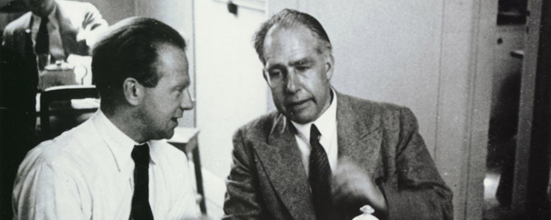













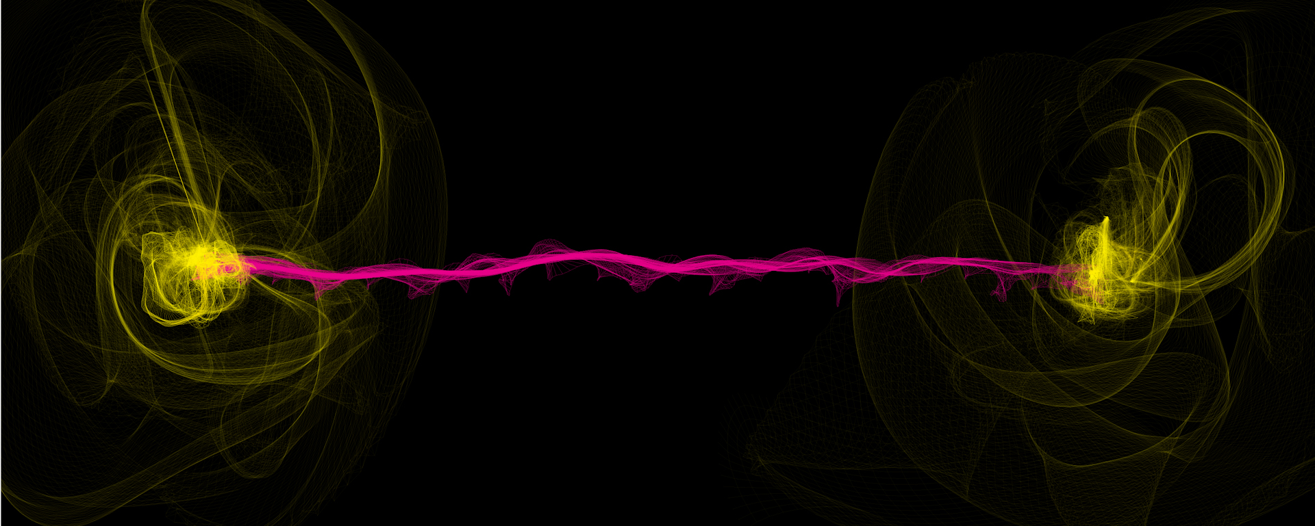





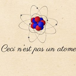

















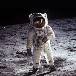













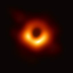

















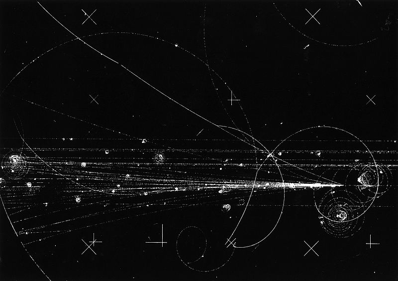









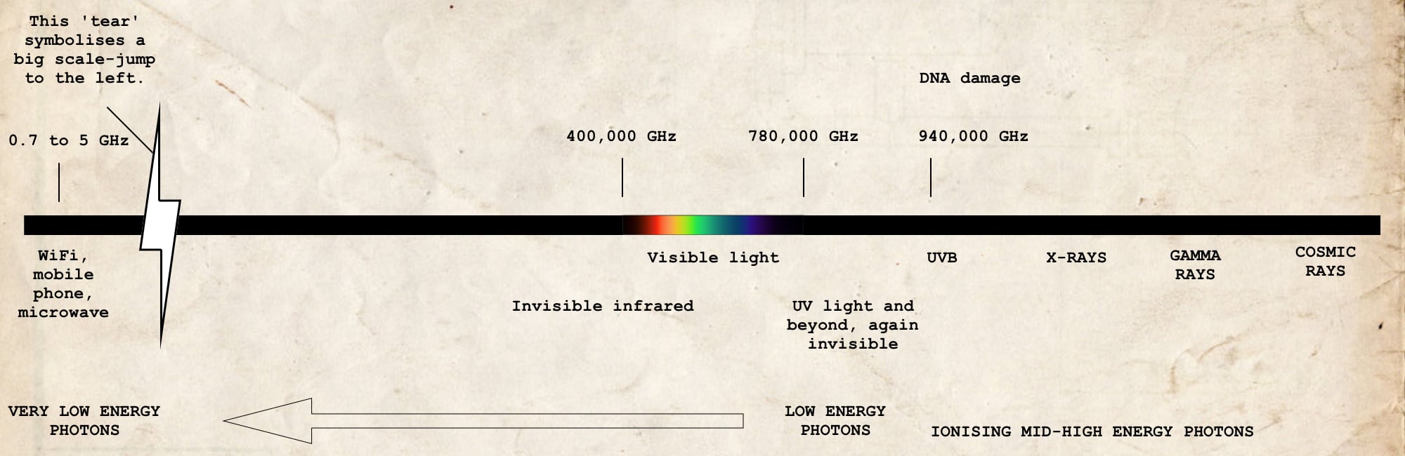
.jpg)