So, you’re reading this post on a quantum mechanical thing, be it a portable device or a less mobile desktop computer. This is all possible because quantum mechanics is the most successful theory humans have been able to conjure up. Nevertheless, there are still a few things to figure out. One of those things is called the measurement problem and sits at the level of a Nobel Prize. Since 1925, one way of solving this was mainly proposed by Niels Bohr and Werner Heisenberg. They coined what is now called the Copenhagen interpretation.
Wave function
Let’s do a quick recap of the mechanics as described in The double-slit experiment. Suppose, we release a bunch of free electrons, meaning that they are not disturbed nor confined by any interaction with any other thing. They are launched from a cannon towards a screen with two slits.
One important element to describe the behaviour of the electron is what is called the wave function (the other element is the Schrödinger equation). It’s a mathematical description of all the possible states the electron can be in as soon as you measure it. In the case of our double-slit experiment, we look at two possible states pertaining to its position: it can be in the position-state of being at slit 1 or it can be in the position-state of being at slit 2.
Figure 1. The screen with slits $\lvert 1 \rangle$ and $\lvert 2 \rangle.$
Let’s use the symbol $\lvert \Psi \rangle$ to denote the wave function of the electron. Indeed, this is the actual notation for the wave function in quantum mechanics. We’ll use $\lvert 1 \rangle$ and $\lvert 2 \rangle$ to denote the position-states slit 1 and slit 2.
So, when we don’t put particle-measuring detectors at both slits, we will not know through which slit the electron will have gone. Quantum mechanics dictates that the wave function of our free electron with respect to its position in space is the addition of the two possible slits it can go through. It is true that it could also bump into the screen, missing the slits. So, let’s label all those positions $\lvert b_n \rangle,$ where $b$ stands for bumping-into-screen and $n$ is a number denoting every tiny position on the screen that is not a slit. The wave function can then be written(beginfootnote)I’m deliberately leaving out any complex coefficients so as to not complicate things for the purpose of this post.(endfootnote) as follows:
Put differently, we say that with respect to its position, the electron is in a superposition of slit 1 and slit 2 and a whole bunch of other positions on the first screen that lead to nowhere but an inglorious end on the first screen.
The unmeasured, free particle is wave-like – going through the two slits at once, spread-out like a wave – as is visible on the second screen: after a while a wave-interference pattern will have emerged.
Figure 2. The typical interference pattern for wave-like phenomena becomes visible on the second screen when free electrons go through the two slits.
Measurement
However, as soon as you attach particle detectors on both slits, the detectors show that the particle only ever goes through one slit. Also, the interference pattern disappears instantly and makes place for your typical particle-like pattern.
The detectors determine or measure the position of the electron to be either at slit 1 or slit 2. Somehow, they never measure the electron to be at slit 1 and 2 at the same time. In other words, its wave-like existence has been replaced by a particle-like existence!
Figure 3. The typical particle-like pattern appears on the second screen as soon as you put detectors at the slits to measure the position of the particle.
The Copenhagen interpretation
Undergraduate students are usually taught the following interpretation of these strange events.
Upon measurement, the particle’s wave function collapses.
That’s it. This is what’s at the heart of the Copenhagen interpretation. This explanation of what’s happening at the act of measurement is named after the city where Niels Bohr worked.
In other words, all the terms of the wave function ‘collapse’ into just one term. Suppose, we measured the electron to be going through slit 2, then by some unknown mathematical operation our wave function
Note that neither the measurement nor the mathematics influence or prescribe at all which terms eventually get cancelled. In this example, it just happens to be that $\lvert 2 \rangle$ was left over. What is eventually being crossed out is fundamentally unpredictable. Moreover, the very process of crossing out is unknown.
The Born rule
Max Born wrote in a Nobel Prize-winning footnote of his 1926 paper that the probability of a solution to the Schrödinger equation of a quantum-mechanical system (such as an electron) is proportional to the wave function squared. A solution to the Schrödinger equation represents a possible specific quantum state, such as being at slit 2. In our equations above, each term represents such a specific quantum state.
So, the only thing we have is the Born rule(beginfootnote)It would have been too cheesy and/or dorky perhaps, but I would have loved Robert Ludlum’s trilogy to at least contain one with the title The Bourne Rule: One Man Against the Odds.(endfootnote), stating that we can only predict the probability of each of the possible terms to not be crossed out after measurement.
Figure 4. The footnote that got Max Born the Nobel Prize[1].
Acceptance of the Copenhagen interpretation
Bohr stated that this collapsing process cannot be described by quantum mechanics. This interpretation seems rather unsatisfactory to many. As the Nobel Prize laureate Steven Weinberg notes, ‘This answer is now widely felt to be unacceptable’[2]. A growing number of physicists realise that one of the problems is that in this case nobody knows what is supposed to be described by quantum mechanics and what not. If wave function collapse oughtn’t fall under the purview of the mathematical formalism, for example, then what criteria should we uphold to determine if something else can be studied quantum-mechanically and what cannot be known, ever?
The major proponents Heisenberg and Bohr stressed that the wave function is purely a mathematical affair. While their views did not always align perfectly, they obviously agreed on wave function collapse[3]. Bohr noted that we had to give up any physical representation of the whole matter. Those who uphold the traditional Copenhagen interpretation are generally instrumentalists.
However, nobody knows if the Copenhagen interpretation is correct. There are other contenders aiming to solve the measurement problem.
We will discuss other instrumentalist and realist interpretations of quantum mechanics in another bit of maths and physics.
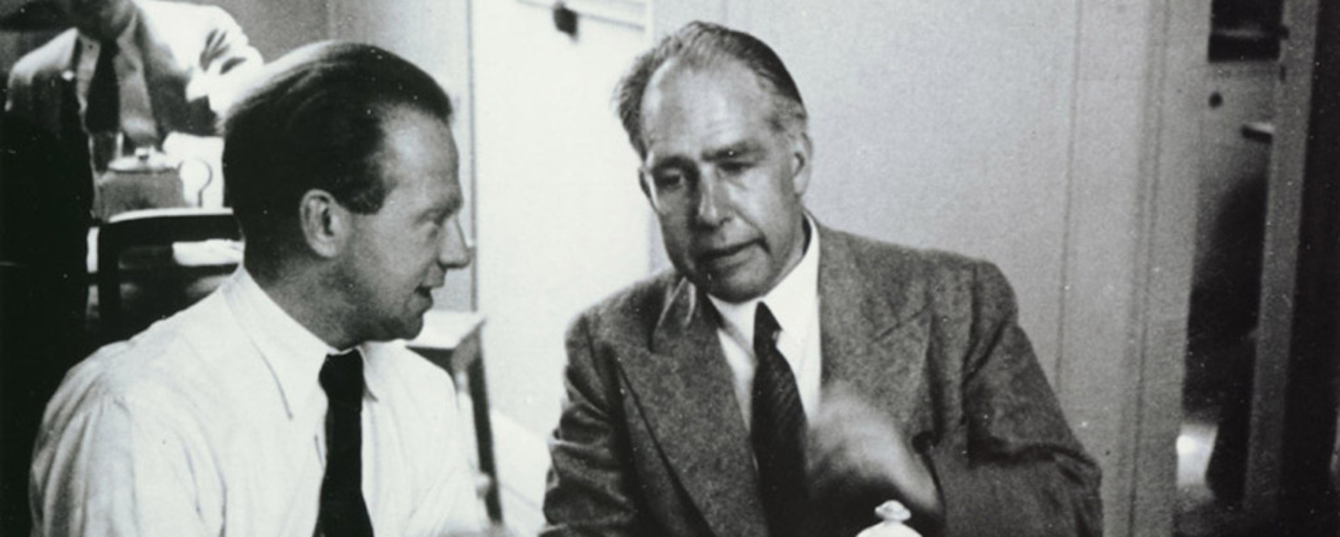
Featured image: Werner Heisenberg (left) and Niels Bohr (right) by Fermilab, U.S. Department of Energy. Public domain.
References
[1] Born, M. (1926) “Zur Quantenmechanik Der Stoßvorgänge,” Zeitschrift für Physik, 37(12), pp. 863–867. doi: 10.1007/BF01397477.
[2] Weinberg, Steven (2018) “14 the Trouble with Quantum Mechanics,” in Third Thoughts. Cambridge, Massachusetts; London, England : Harvard University Press, 2018, pp. 124–124.
[3] Kiefer, C. (2003) “On the Interpretation of Quantum Theory — from Copenhagen to the Present Day,” in Castell, Lutz and Ischebeck, Otfried (eds.) Time, Quantum, and Information. Berlin; New York : Springer, 2003, pp. 291–299. doi: 10.1007/978-3-662-10557-3_19.
The last few posts on quantum mechanics have been quite extensive and at times rather deep for those who are on the move. So, here are ten important ideas about particles and wave functions for when you’re en route in slightly more normal English.
To describe objects in our everyday world, such as rocks, buildings, and cars, Newton’s laws suffice. To describe subatomic, elementary particles, such as electrons, protons, neutrons, and photons, however, there is a whole different type of physics: quantum mechanics.
2: Wave functions
The most complete description of an elementary particle is called the wave function. Actually, the word ‘particles’ seems to incorrectly refer to tiny points, balls or spheres or something, which they are absolutely not. They aren’t waves either. ‘Particles’ are wave functions with wave-like properties (emphasis on ‘like’). Upon interaction with other particles and/or measurement, they exhibit particle-like behaviour, however. The wave function contains all physically possible states a ‘particle’ can be in at the moment we measure its state. The wave function can be seen as a mathematical description of the probabilities of the states that the particle will snap into as soon as you measure it. It’s often visualised as a ‘cloud’ even though that’s not what it actually looks like. It’s just a visual metaphor for a mathematical object that actually lives in complex space as it is complex valued.
I usually just draw vague spherical thingies.
3: Quantum state
Once measured, particles show one specific quantum state out of a whole range of possible quantum states prior measurement. Position is the most intuitive to understand example of a quantum state. Momentum is another (momentum is a measure of the amount of motion of a particle). Then there are states such as polarity, spin, and a bunch of others. The wave function encapsulates all these possible states and yields a probability-value for actually measuring a particular state. In other words, even before you measure it, the wave function allows you to calculate the chances of encountering this particular quantum state.
4: Measurement problem
As long you don’t measure a particle, and as long as it doesn’t interact with other particles, the particle is not in a specific quantum state yet. Instead, its wave function just describes all these possible states as though they are mathematically added on top of each other. This ‘adding of quantum states’ is what is meant when physicists talk about superposition. The term is from the mathematics of waves and linear algebra in general, not quantum mechanics in particular. While the situation is often portrayed as particles being in multiple states all at once (such as being in two positions at the same time), it’s more accurate to say that the particle does not have a specific state at all. There’s just the wave function with all the probabilities of future quantum states. As soon as you perform a measurement, the particle snaps out of its wave function full of possibilities into a single possibility. In other words, what you see is not what it was. What you observe is just a sliver of its total prior existence. How this happens, nobody knows. It’s called the measurement problem. There’s a Nobel Prize waiting for you.
This extraordinary experiment yielded a photo of the closest approximation of the wave function of an electron in a hydrogen atom we have to date. It was made by the Polish physicist Aneta Sylwia Stodolna et al. (Source: Stodolna AS et al. (2013) “Hydrogen Atoms Under Magnification: Direct Observation of the Nodal Structure of Stark States,” Physical review letters, 110(21), pp. 213001–213001.)
5: Schrödinger equation
Wave functions obey the Schrödinger equation. You could say that what Newton’s second law is for objects in our everyday world, is what the Schrödinger equation is for the subatomic world. It gives us the ability to predict how the wave function evolves in time. This is a completely classical equation; it is 100% deterministic. Where the wave function captures a range of probabilities, the Schrödinger equation tells us how this range of probabilities changes over time perfectly predictably so. In other words, it doesn’t predict the exact state of a particle once measured, but it does accurately predict the probability-value of an exact state once measured at any given time.
6: Uncertainty
There is a fundamental informational trade-off between certain possible states such as between position and momentum, energy and time, and time and frequency. The origin for this does not lie in quantum mechanics. It’s due to the way they are related to each other. Mathematically, these variables are called Fourier transform pairs or conjugate variables. To calculate one from the other, you have to execute a mathematical procedure called a Fourier transform. The trade-off is that Fourier transforming a variable whose range of possible values is smaller leads to the other variable having a larger range of possible values. And if a range of possible values becomes larger, then the exact outcome of measurement is less certain (the probability of a specific state after measurement becomes more uncertain). Heisenberg showed that this uncertainty principle also applies to the wave function in quantum mechanics, hence, there the principle is called Heisenberg’s uncertainty principle.
Fourier showed that if a sound is fairly well-defined in time (bottom), it has to be comprised of multiple frequenties (illustrated as multiple waves at multiple frequencies). That’s the fundamental uncertainty principle with waves.
7: Certainty
That same principle predicts that, while very valid at the scale of subatomic particles, this uncertainty becomes utterly meaningless at our large-scale world of everyday objects. A bowling ball whose range of possible positions is very limited (locked in a very tight enclosure with little to no leeway), will never portray any uncertainty values pertaining to its motion (momentum), for instance. By Heisenberg’s uncertainty principle, upon measurement, it might show to have the speed of $3.283 \times 10^{-35} \text{ m/s}.$ This means that after 965.9 billion years it will have travelled the distance of the width of a proton. So, no, uncertainty effects play no role in our everyday world, unless you are doing experiments with a running time of seventy times the age of our current Universe. In that case, you will have to deal with the uncertainty of the width of a proton(beginfootnote)When people state or think that everyday objects (our bodies, brains, tennis balls, animals) can exhibit quantum effects such as being at multiple places at the same time, I suspect this is because they have no well-defined idea how small subatomic particles really are and no inkling as to how large the everyday world is in those terms. Also, they didn’t do the calculations.(endfootnote). We do note that extraordinarily sensitive larger-scale equipment such as the the mirrors at the LIGO and Virgo experiments are capable of measuring quantum effects, however, this isn’t really unexpected nor is it the same as saying a human body is in a quantum superposition. Measuring quantum effects is one thing, brains supposedly being in two places on Earth (‘based on principles from quantum mechanics’) is a whole other thing.
Missing the pins has nothing to do with practical nor theoretical quantum effects. You’re just not that good.
8: Quantum entanglement
When two or more particles can only be described by one wave function – not as separate wave functions – those particles are said to be quantum entangled, either partly or completely. A measurement performed on one particle immediately determines the measurement outcome on the other entangled particle, irrespective of the spatial distance between them. This is why this phenomenon is said to be non-local. How this happens, is unknown. This effect dissipates to zero when entangled particles interact with yet other particles. At the large scale of our everyday world, the number of particles inside an object to be interacted with is so great, quantum entanglement completely fades away. In very special conditions, however, such as in our labs, entanglement can be sustained for quite some time.
This isn’t what quantum entanglement looks like. It’s just a picture.
9: Quantum Field Theory
Over the years, the mathematical and physical theory of (quantum) wave mechanics has been extended to describe quantum fields as the fundamental building blocks of our Universe. The Universe is made of quantum fields. The most complete description of fields are wave functions. This is called Quantum Field Theory (QFT). The most successful version of QFT is called the Standard Model of quantum physics. ‘Particles’ are here some kind of disturbance in their field: an electron is a disturbance in the electron field. The particle’s description is here part of the wave function of its entire field. The challenge is now to extend this quantum field theory into its next form, encapsulating something called quantum gravity. What we don’t know yet, for example, is how to have space and time in extreme regions such as black holes, naturally appear out of a quantum theory.
My very sketchy way of showing quantum fields. Proton field is not really a thing. It’s just a shortcut for several quark fields. Besides, fields aren’t two-dimensional, they’re obviously three-dimensional.
10: Applications
While the famous physicist and Nobel Prize winner Richard Feynman is known for having said, ‘I think I can safely say that nobody understands quantum mechanics’, this is sometimes incorrectly taken to be a reason to state that, therefore, physicists don’t know what they’re talking about. Feynman alluded to the fact that there is much we don’t know about the foundations of quantum mechanics. There is still much employment in solving hard problems such as quantum gravity, the measurement problem, the strong CP problem, the interpretation of quantum mechanics, non-locality, and so forth.
On the other hand, we now have WiFi, internet, touchscreens, lasers, MRI scanners, LEDs, flash memory, solid state disks, the old crunchy hard disks, transistors, and CPUs or integrated chips (ICs) in general.
I think I can safely say that the fact that you’ve plucked this article out of the air to have it displayed on your (touch)screen is at least an indication of the level at which ‘nobody understands quantum mechanics’.
Nevertheless, we’re far from done. There is still much to discover in this Universe with a bit of maths and physics.
It’s perhaps not as famous as Einstein’s formula but in this day and age many people may still have heard at least once of the phrase ‘Heisenberg’s uncertainty principle’. It plays an important role in quantum mechanics. You may have heard that every time you observe or measure matter, due to the crudeness or inherent inaccuracy of the measurement device, you will inevitably disturb your own observation. This would then preclude you from gaining accurate knowledge with satisfying certainty. In fact, in general, Heisenberg’s uncertainty principle states that nothing can be certain. At the risk of sounding vague and vanilla, all of these statements are completely and utterly wrong. Let’s look at what it really says, shall we?
Figure 1. Werner Heisenberg in Göttingen in 1924.
Fourier transform pairs
Trade-offs. Who doesn’t hate them? Remember when your parents told you that you could have this but then not have that or maybe just a bit of this but then less or fewer of that? Unsurprisingly, at least three famous philosophers have written a few words on this, each in their own way lamenting on the existence of trade-offs and how to deal with them. One chose to become all rebellious about it and wrote: ‘I want it all, I want it all, and I want it now!’ (May, 1988). The other two, however, chose to be more pragmatic about it as they postulated that ‘you can’t always get what you want’ (Jagger & Richards, 1968). Obviously, they knew that, sometimes, life brings you Fourier transform pairs. The more well-known example is of course Heisenberg’s uncertainty principle.
If you limit a particle’s range of possible positions in space $(\Delta x)$, you increase its range of possible momenta(beginfootnote)Momentum is the product of mass $m$ and velocity $v,$ so $p=mv.$ It’s a measure for the amount of motion of an object.(endfootnote) along the $x$-direction $(\Delta p_x),$ and vice versa.
This is formalised as follows:
$$\Delta x \Delta p_x \geq \frac{\hbar}{2}.$$
Just to be absolutely clear: the delta-symbol $\Delta$ is a range of a certain quantity. Usually, a $\Delta$ is defined as the difference between two values. Suppose, you measure point $A$ of your garden fence to be $0.1$ metre away from your wall and point $B$ to be $0.7$ metre away from your wall, then the $\Delta$ of the distances, i.e. the length between points $A$ and $B,$ is $0.7-0.1=0.6$ metre.
In Heisenberg’s principle, it is stated that the product of the range of possible positions $\Delta x$ and the range of possible momenta $\Delta p_x$ is greater than or equal to some number. Mind you, it’s a tiny number. The symbol $\hbar$ stands for the Planck constant divided by $2 \pi,$ and the result gets cut in half yet again.
This means that whenever one is getting bigger, $\Delta p_x$ for instance, the other is getting smaller, which is then $\Delta x.$ And vice versa.
Click here if you’d like to do a bit of maths. It’s very easy.
Just to get an intuitive insight in this relation, suppose $\frac{\hbar}{2}=1,$ and so, suppose, $\Delta x \Delta p_x = 1.$ Furthermore, suppose $\Delta x = 0.5.$ What value does $\Delta p_x$ has to be to satisfy this equation? Exactly, $\Delta p_x$ has to be $2,$ because $0.5 \times 2 = 1,$ or else the equation is false.
Now, lets make $\Delta x$ smaller. In other words, we’re going to try to pinpoint the location with much more precision. So, let’s say, $\Delta x = 0.001.$ What value does $\Delta p_x$ has to become to satisfy this equation? You guessed right, $\Delta p_x$ has to become even larger: $\Delta p_x = 1000,$ because $0.001 \times 1000 = 1.$ If you were to reverse the situation – decreasing the size of $\Delta p_x$ – then, in turn, $\Delta x$ would have to become larger.
In reality, $\frac{\hbar}{2}$ is much smaller than 1. It is, in fact, about $5.273 \times 10^{-35} \text{J/s}.$ That’s thirty-four zeros behind the decimal point and then ending in 5273. It’s incredibly small. Don’t worry about this. We’ll get back to that later.
Hopefully, now you see the relation between $\Delta x$ and $\Delta p_x$ as put forward by Heisenberg’s formulation. They complement each other. Whenever a range of possible values becomes larger, in other words, the $\Delta$ or range of value-options is larger – its actual value becomes more uncertain, hence the use of the word ‘uncertainty’ in Heisenberg’s uncertainty principle(beginfootnote)In fact, it’s statistics. The $\Delta$-sign could just as well be a $\delta$-sign, so $\delta x \delta p_x \geq \frac{\hbar}{2},$ which signifies its statistical character more accurately. After all, the wave function is about probabilities.(endfootnote).
But why is this? While this principle plays a central role in quantum mechanics, it’s actually not fundamentally a quantum-mechanical law. This principle exists more generally in many instances in physics, and, even more generally, in mathematics.
In mathematics, the variables position and momentum are said to be a Fourier transform pair. Put in yet other mathematical jargon, position and momentum are said to be conjugate variables.
Sound
A well-known, non-quantum-mechanical example of the uncertainty principle is determining the pitch of a sound. How ‘high’ a note is, depends on the frequency.
The most familiar way we depict sound waves is a simple sine wave. It represents the simplest of sounds possible. Also, it’s the most boring of sounds possible.
The $x$-axis represents time. The $y$-axis represents the amplitude of the sound or the loudness, the intensity of it. As you can see, the sound wave repeats itself over time; the pattern is cyclic. One whole cycle is when the plot has completed going up, going down, going further down, and going up again. The time it takes to complete one cycle is designated by the symbol $T,$ called the period(beginfootnote)It is also possible to measure the time-distance between two peaks or two troughs.(endfootnote). So, this particular sound wave is said to be periodic.
Figure 3. A time-amplitude plot of a boring old sinusoidal sound wave. (Click to enlarge.)
The shorter the period – the quicker the cycles are – the higher the tone. Another way of saying, is that the higher the frequency, the higher the tone. The mathematical relationship between period $T$ and frequency $f$ is the following expression:
$$f = \frac{1}{T}.$$
If the period gets shorter, i.e. the value of $T$ becomes smaller, then the value of $f$ becomes larger, which means higher, which means a higher tone.
Seeing as the time period $T = 2 \pi$ seconds, the frequency diagram looks like a spike at $\frac{1}{2 \pi}$ Hz. In this frequency-diagram, the $x$-axis is the frequency and the $y$-axis is still the amplitude.
Figure 4. A frequency-amplitude plot of the sound wave of Figure 3. It shows the exact frequency at which that sound wave exists.
So, there are now two ways in which we can describe the sound wave: either by frequency (Figure 4) or by change over time (Figure 3).
Notice that the sound wave plotted as a function of time (Figure 3) has no beginning nor end. For all we know, that plot could just go on forever, to an infinite amount of time, in both directions. Suppose, we would ask the question at what time exactly does the sound exist? The answer is: always. There is no particular, specific time at which it exists.
In other words, we could write that $\Delta t = \infty.$
Notice, however, that the frequency plot looks very finite: just one stroke. One well-defined, finite stroke. If we were to ask the question what frequency exactly does the sound have? The answer is: there is a particular, specific, exact frequency at which it exists and it is $\frac{1}{2 \pi}$ Hz $( \approx 0.16).$
Fourier analysis
In reality, no sound is going to be infinitely long. Pluck a guitar string and it will fade out as the energy dissipates slowly. Also, at some point it started – meaning, before that, it didn’t exist. In other words, in reality, a sound wave usually exists in a finite range of time.
Let’s limit our sound wave to a range in time, so it looks more like the sound of a ‘blip’ and less like an infinite tone of boredom. Again, the $x$-axis represents time and the $y$-axis represents the amplitude.
Figure 5. A time-amplitude plot of a so-called wavelet, a short sound burst. Contrary to the sound wave in Figure 3, it’s not infinitely long. It’s now also more difficult to assess its frequency.
As you can see, the sound now exists in a more defined range of time – roughly 1.5 seconds. In other words, $\Delta t \approx 1.5$ seconds. That’s a whole lot smaller than the old $\Delta t = \infty.$
Now, we ask ourselves, what is its frequency? The difficulty now is that it’s hard to pinpoint an exact period $T$. The evolution of the plot is quite different from our infinitely long sine wave. Yes, we can identify kind of those cycles we’re looking for, however, no cycle has the same shape, so, technically, we’re dealing with multiple cycles at once. And guess what, its frequency-amplitude plot looks like this.
Figure 6. The frequency-amplitude plot of the wavelet in Figure 5. It’s far from being a specific, exact frequency. At varying degrees, it’s actually a few frequencies at the same time.
As you can see, it has become difficult to pinpoint the exact frequency of our wavelet. It exists at a variety of frequencies and amplitudes.
So, while the ‘time window’ of the sound wave has become more exact, the frequency has now become ‘less certain’.
The brilliant mathematician Joseph Fourier discovered that a wavelet such as in Figure 5 can actually be constructed by adding many infinite waves at many frequencies. Put differently, Fourier analysis shows that our wavelet is the culmination of a superposition of many waves at many frequencies.
Figure 7. The wavelet at the bottom is constructed by many infinite waves at many different frequencies superposed onto each other. This automatically means that the wavelet’s exact frequency is fundamentally harder to determine than the frequency of the sound wave in Figure 3.
Now you see why the frequency-amplitude plot has changed from a very specific value in Figure 4 to the wider set of frequencies in Figure 6. In the latter case, the wavelet ‘contains’ multiple waves at multiple frequencies, so when you Fourier transform its time-amplitude plot to its frequency-amplitude plot, the frequency has become ‘uncertain’.
The relation between time $\Delta t$ and frequency $\Delta f$ in ordinary classical physics is fundamentally complementary. No quantum mechanics needed.
The term ‘Uncertainty principle’ pertains to the general phenomenon that Fourier transforms (such as between time and frequency) entail a fundamental, mathematical trade-off between types of information carried by the two transformed variables. Heisenberg then showed that this principle also holds in quantum mechanics. And so, the uncertainty principle in quantum mechanics is called Heisenberg’s uncertainty principle.
The De Broglie relation
Time to go back to quantum mechanics. Remember that a particle’s best description is a wave function? A wave function is the mathematical expression of a particle containing all possible states it can assume once we measure it.
Instead of a time-amplitude plot, let’s represent a particle by a space-amplitude plot. To make it a little bit easier, let’s take the wave function of a particle of which the amplitude only varies along one dimension of space, $x.$
Here is a representation of a particle’s wave function along one dimension of space (along a ‘straight line’). The $x$-axis represents a position in space. The $y$-axis represents the amplitude of the wave function (which is proportional to the probability of finding the particle in that particular position $x$).
Figure 8. A representation of a wave function of a free particle. Note that this is not what it actually looks like. For one, an actual wave function exists in complex space, which we didn’t plot here. The goal is to illustrate, not to map accurately. Also note that the free particle has no specific position yet as it’s a free particle!
It was the eminent French physicist Louis de Broglie(beginfootnote)Many physicists have tried and mispronounced his last name. It should sound like ‘broy’ where the r is produced at the back of the throat, like the French r – a ‘dry’ kind of r. In this interview with him, you can hear the French presenter pronouncing his name (just after 0:16 seconds). It’s not ‘brog-ly’ nor ‘bro-ly’. Thank you.(endfootnote) who formulated the relationship between a particle’s wave function’s wavelength $\lambda$ and its momentum $p.$
$$\lambda = \frac{h}{p},$$
where $h$ is the Planck constant. Incidentally, this is the equation better known as De Broglie’s matter wave hypothesis, stating that matter, such as electrons, possess a wave-like characteristic(beginfootnote)Do note that this same equation shows that this wave-like behaviour of large bodies such as our bodies, brains, bowling balls, tennis balls, and animals is completely and utterly negligible as we will demonstrate at the end of this post.(endfootnote). This won him the Nobel Prize, no less.
If we rewrite this to solve for $p,$ we get
$$p = \frac{h}{\lambda}.$$
So, clearly, a wave’s momentum is determined by its wavelength. The smaller the wavelength, the greater the momentum. What is the wavelength? It’s the length between two peaks (or two troughs). The higher the frequency, the smaller the wavelength. Now have a look at Figure 8 again. As you can see, the infinite wave of a free particle has a well-defined wavelength. The logical conclusion is that the momentum is also well-defined. Nevertheless, Figure 8 also shows that the particle’s position is not defined at all!
Let’s turn this on its head and limit the range of possible positions of our particle. No longer is it a free particle. It is now confined within a finite range of locations.
Figure 9. Our former free particle’s position is now restrained between $x = 0$ and $x= \pi.$ In other words, $\Delta x$ is now limited to $\pi$ wide. There is no well-defined wavelength as the wave function has different values in different places. It’s there, but not as well-defined as in the wave function in Figure 6.
What we’ve done in Figure 9 is making $\Delta x$ smaller than it was in Figure 8 (where it was infinitely large). In fact, $\Delta x = \pi$ wide. By the same Fourier transform mechanism as with the time-frequency pair, the complimentary sister of position space $\Delta x$, namely momentum space $\Delta p_x$, will now become less certain.
To construct a limited wave function such as the one in Figure 9, Fourier analysis shows that you need – again – a bunch of waves at different frequencies in superposition (added on top of each other).
Figure 10. A Fourier deconstruction of the wave function in Figure 9. Many waves, many frequencies. Hence, the momentum is less well-defined.
So, when it comes to quanta, Heisenberg’s uncertainty principle states that there’s a fundamental trade-off between information on position and momentum(beginfootnote)Another pair is energy and time. This is interesting in the context of Hawking radiation. We’ll get to that, don’t worry.(endfootnote). This is due to the fact that they are a Fourier transform pair or conjugate variables.
This also means that if you constrain a particle to a minuscule $\Delta x,$ its wave function will start to contain momenta $\Delta p_x$ all over the place. It will occupy many more velocity possibilities, including the much faster velocities. If you were to subsequently perform a measurement, the probability of finding it moving at higher speeds is now much larger!
Scale and effect
At the scale of the big bad world, we never see this effect. If you would confine a bowling ball in a limited space, you will not see its momentum increase dramatically. It won’t suddenly start bouncing up and down. Conversely, if you swoop the bowling ball with considerable momentum, it won’t suddenly start appearing everywhere and nowhere at the same time: its position is still quite clear. You won’t suddenly quantum tunnel through the pins or be rolling on all bowling lanes of the neighbouring players at the same time. If it doesn’t hit a single pin, then that’s not because it’s suddenly in a state of superposition with regard to its possible locations of existence. You’re just not that good.
You won’t notice any of these quantum effects in your everyday-scaled objects. Only when you’re dealing with particles. Or atoms. However, as soon as the mass increases, it all changes. Why? Partly because Planck’s constant is so darn small(beginfootnote)And because the number of interactions between atoms increase exponentially, causing any quantum effect to disappear due to decoherence.(endfootnote). It’s just $5.273 \times 10^{-35} \text{ J/s},$ remember? That’s small.
All this knowledge does allow for some fun calculations. For instance, if you were to confine a bowling ball with a mass of $7.2$ kg (16 lb) inside a box where $\Delta x = 22$ cm (8.66 inches), by Heisenberg’s uncertainty principle, the ball’s speed will be $3.283 \times 10^{-35} \text{ m/s}.$ That means that after $965.9$ billion years it might have moved a distance equal to the diameter of a proton. That amount of time is seventy times the age of our current universe. Granted, quantum-mechanical effects aren’t zero, but as you can see (or rather, as one can calculate), on our everyday scale, these effects are quite meaningless.
Sometimes, weird films such as What the #$*! Do We (K)now!? and What the Bleep!?: Down the Rabbit Hole will want to make you believe such quantum things can happen anyway. They will mention Heisenberg’s uncertainty principle like it is a magical law allowing us to do whatever. I hope that this post has shown that Heisenberg’s uncertainty principle is not about that. Nor does the uncertainty principle itself have its roots in quantum mechanics. It’s basically wave mechanics, the classical stuff, which all first-year undergraduates in physics have to learn in their first or second semester.
A few months ago, I stumbled across a video showing an Australian senator’s question to the head of the Commonwealth Scientific and Industrial Research Organisation, an Australian federal government agency responsible for scientific research. Clearly, the senator had – shall we say ‘read something about Heisenberg’s uncertainty principle’. During a senate hearing for a legislative committee, the senator questioned if research done in climate change should be taken with precaution as Heisenberg’s uncertainty principle stands in the way of accurate measurements(beginfootnote)He basically sought a ‘scientific’ way to put climate science in doubt – which, apparently, he is not a proponent of. I do not claim to know anything about Australian politics, or even at great depth about climate science, however, when a legislator starts talking quantum physics – well, I do know stuff about that.(endfootnote).
I suspect this discussion pertained to a study where a satellite uses infrared radiation to perform surface and/or atmospheric remote sensing. He continued to state that as infrared light has lower frequencies than visible light, it’s ‘very difficult’ to understand the properties of infrared radiation based on Heisenberg’s uncertainty principle.
Many things were going on (wrong) in this one short bit of speaking time of the senator, as is usual when someone hasn’t caught up on quantum physics as much. Which is understandable, but no less gnawing to watch (the link opens a new tab and leads to a short video on Twitter).
In any case, I genuinely hope that this article contributed at least a sliver of knowledge to educate the electorate of the world, so we can all vote as informed and responsible as possible for the right persons for the right jobs, besides one’s preferred socioeconomic idealism.
If you should take one thing from this post, it’s that Heisenberg’s uncertainty principle is not about anything spiritual nor does it have anything to do with scientific measurement mistakes: it’s good, old wave mechanics and Fourier analysis taught to undergrads in their first year at university. It works and it works well. It does not lead to science not being able to know things about the universe. In fact, it increased our knowledge of it. In fact, no modern information device would have worked without it. After all, you’re reading this with an electronic device which exists thanks to Fourier, Heisenberg, and De Broglie, among others. All that with a bit of more maths and more physics at the same time.
Photo Werner Heisenberg by Friedrich Hund, a German physicist who took this photo in Heisenberg’s place of residence, Göttingen, in 1924. It was uploaded to Wikimedia Commons under CC BY 3.0 by Friedrich Hund’s son, Gerhard Hund, a German mathematician, computer scientist, journalist, and chess player. We have used a colour-corrected version by Martin Geisler.